Ideally, we should use distribution that can effectively separate three key parameters: Difficulty, Onset, and Scale…
Expertise
lme4
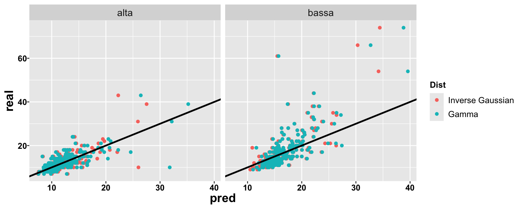
Gamma vs. Inverse Gaussian
Gamma
α > 0 shape
λ > 0 rate
Inverse Gaussian
μ > 0 mean
λ > 0 shape
Their are both difficulty-like parameter: μ = α / λ,
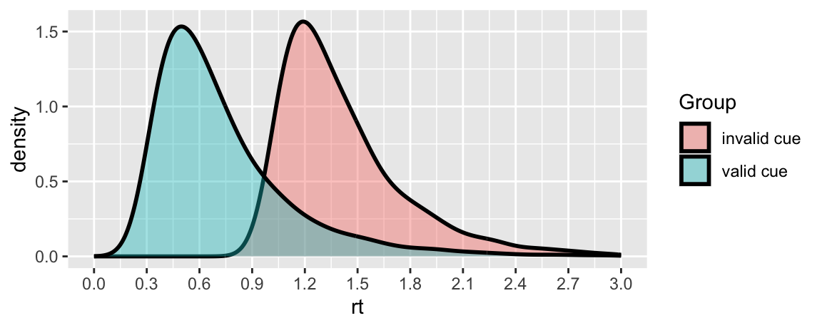
μ reflects difficultyμ = μ , λ influence the scale. The larger μ and the smaller λ, the more variable the RTs:
Gamma
Interpretability
α independent events.
λ rate of events per unit time.
The total time for all events follows a Gamma distribution
Inverse Gaussian (Wald)
Interpretability
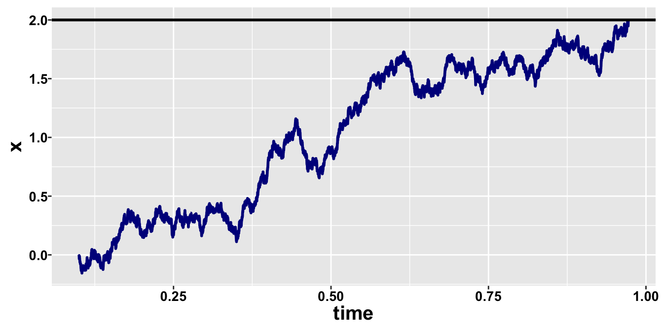
The name “inverse Gaussian” comes from its relation to Brownian motion (or Wiener process). It “describes the distribution of the time a Brownian motion with positive drift takes to reach a fixed positive level” [Wikipedia].
Code
set.seed(11)rdm_path =function(drift, threshold, ndt, sp1=0, noise_constant=1, dt=0.0001, max_rt=2) { max_tsteps = max_rt/dt# initialize the diffusion process tstep =0 x1 =c(sp1*threshold) # vector of accumulated evidence at t=tstep time =c(ndt)# start accumulatingwhile (x1[tstep+1] < threshold & tstep < max_tsteps) { x1 =c(x1, x1[tstep+1] +rnorm(mean=drift*dt, sd=noise_constant*sqrt(dt), n=1)) time =c(time, dt*tstep + ndt) tstep = tstep +1 }return (data.frame(time=time, x=x1, accumulator=rep(1, length(x1))))}drift =1;threshold =2; ndt = .1sim_path =rdm_path(drift = drift,threshold = threshold, ndt = .1)ggplot(data = sim_path, aes(x = time, y = x))+geom_line(size =1, color ="blue4") +geom_hline(yintercept=threshold, size=1)
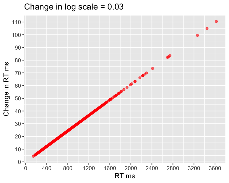
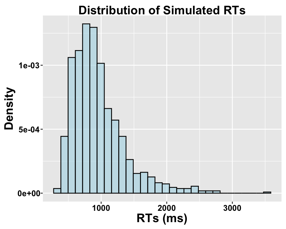
Logarithms model proportional changes rather than absolute differences.
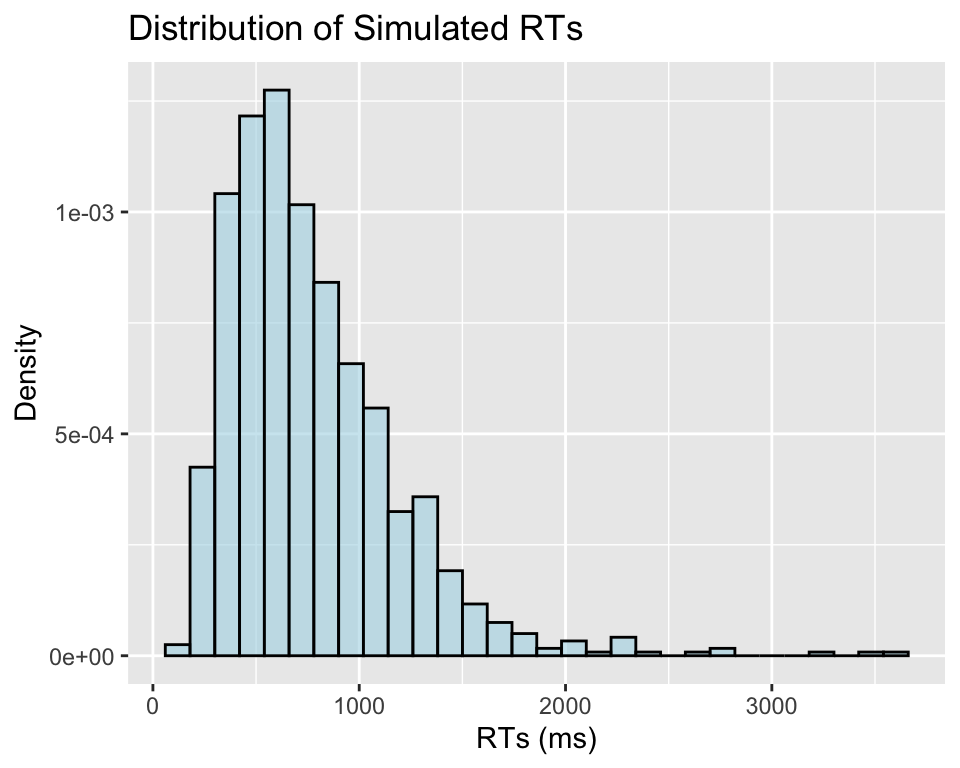
Code
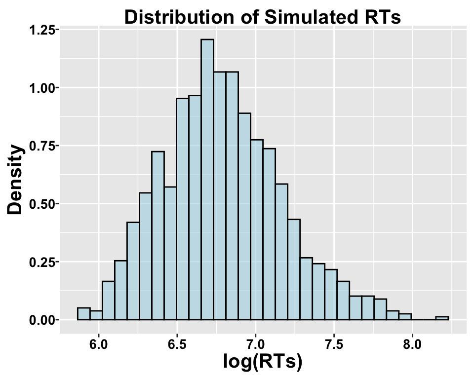
# Set seed for reproducibilityset.seed(123)# Parameters for simulationn =1000# Number of observationsa =6.5# Baseline intercept for the log-transformed mean (mu)b =0.02# Effect of covariate Xx =rnorm(n, 0, 0.05) sigma =0.5# Standard deviation of the log-transformed RTsmu = a + b*x# Effect of X on mu (mean log RT)RT =rlnorm(n, meanlog = mu, sdlog = sigma) # Log-normal dataggplot(data.frame(rt = RT), aes(x = rt)) +geom_histogram(aes(y = ..density..), bins =30, fill ="lightblue", color ="black", alpha =0.6) +labs(title ="Distribution of Simulated RTs", x ="RTs (ms)", y ="Density")
Code
RT_diff =exp(log(RT) +0.03) - RT ggplot(data.frame(mu = RT, relative_change = RT_diff), aes(x = mu, y = RT_diff)) +geom_point(alpha =0.6, color ="red") +labs(title ="Change in log scale = 0.03", x ="RT ms", y ="Change in RT ms") +scale_x_continuous(breaks =seq(0,4000,400))+scale_y_continuous(breaks =seq(0,120,10))
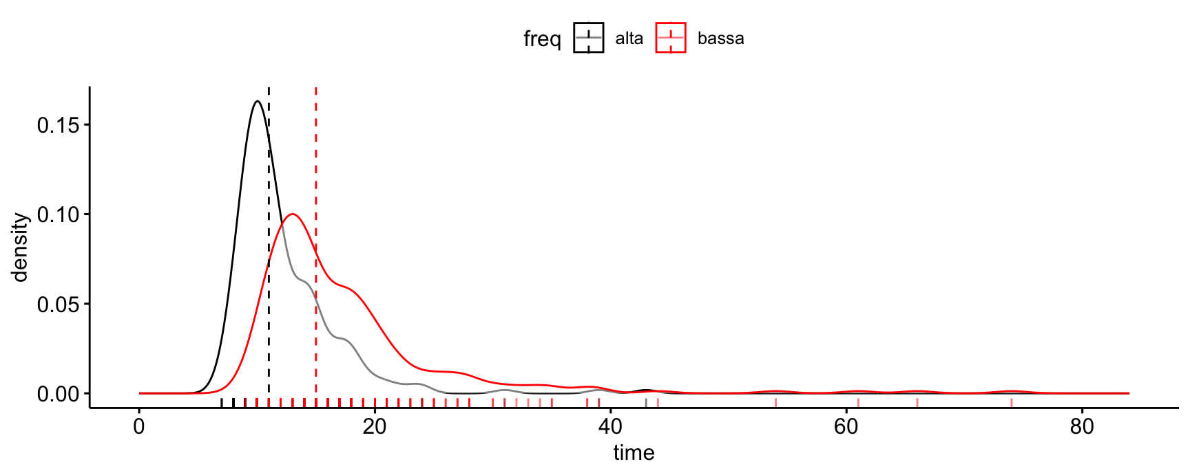
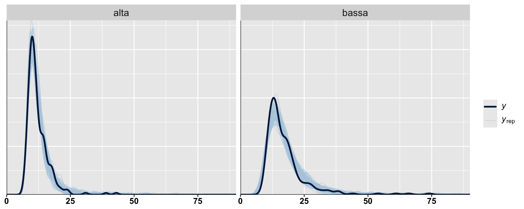
Reading time
High frequency vs. low frequency words, children 9-15 y.o.
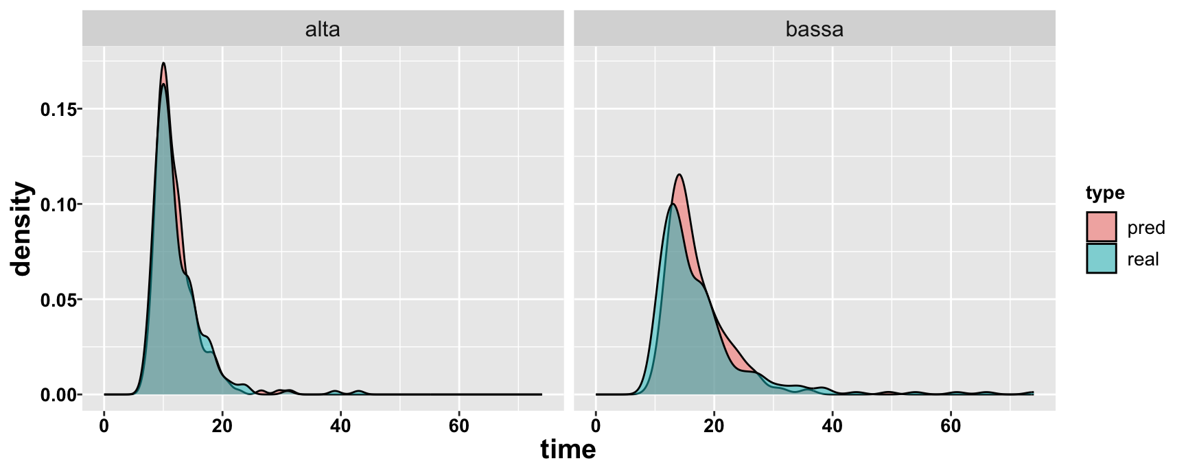
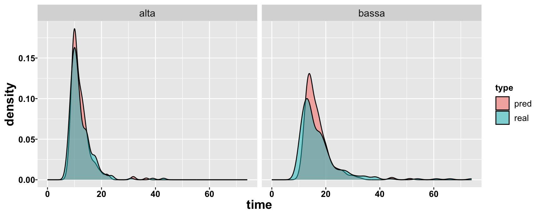
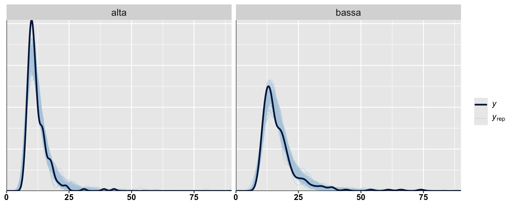
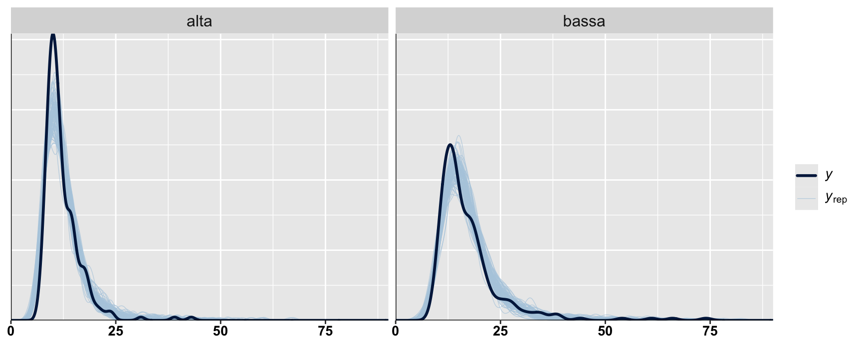
Inverse Gaussian vs. Gamma
Code
mInv = lme4::glmer(time ~ freq + age + (1|ID), data = dat_e, family =inverse.gaussian(link ="log"))sumInv =summary(mInv)mGam = lme4::glmer(time ~ freq + age + (1|ID), data = dat_e, family =Gamma(link ="log"))sumGam =summary(mGam)
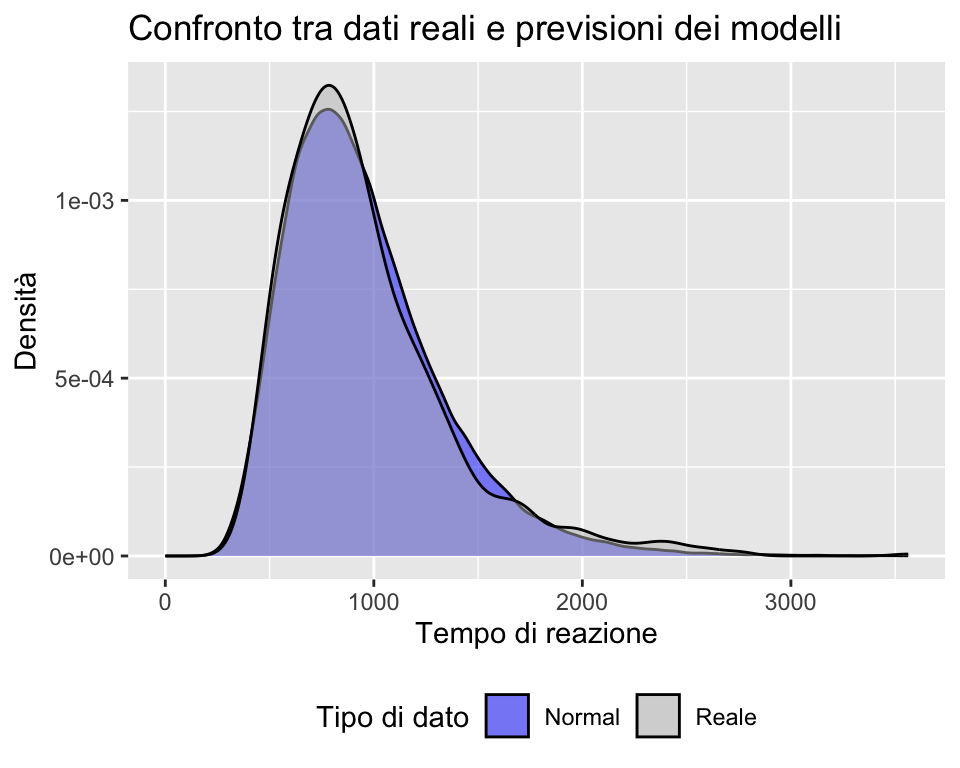
If Y is log-normally distributed, then log(Y) follows a normal distribution. The distribution is defined directly for Y, not for a transformed version of Y!
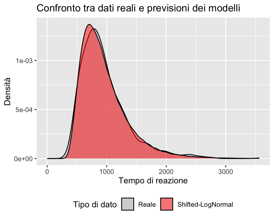
- influence difficulty. Median = shift + exp(μ).
σ > 0 scale - increases mean = (but not the median).
Warning: There were 144 divergent transitions after warmup. Increasing
adapt_delta above 0.8 may help. See
http://mc-stan.org/misc/warnings.html#divergent-transitions-after-warmup
 Family: shifted_lognormal
  Links: mu = identity; sigma = identity; ndt = log
Formula: time ~ freq + age + (1 | ID)
         ndt ~ 1 + (1 | ID)
   Data: dat_e (Number of observations: 476)
  Draws: 4 chains, each with iter = 6000; warmup = 3000; thin = 1;
         total post-warmup draws = 12000

Multilevel Hyperparameters:
~ID (Number of levels: 238)
                  Estimate Est.Error l-95% CI u-95% CI Rhat Bulk_ESS Tail_ESS
sd(Intercept)         0.51      0.04     0.43     0.59 1.00     2310     5146
sd(ndt_Intercept)     0.16      0.03     0.09     0.22 1.01      539     1355

Regression Coefficients:
              Estimate Est.Error l-95% CI u-95% CI Rhat Bulk_ESS Tail_ESS
Intercept         1.76      0.10     1.55     1.95 1.02      675     1355
ndt_Intercept     1.95      0.07     1.81     2.07 1.01      617     1389
freq1            -0.74      0.07    -0.89    -0.62 1.01      796     1754
age              -0.22      0.04    -0.31    -0.14 1.01     1225     2948

Further Distributional Parameters:
      Estimate Est.Error l-95% CI u-95% CI Rhat Bulk_ESS Tail_ESS
sigma     0.31      0.03     0.26     0.37 1.01     1454     3114

Draws were sampled using sampling(NUTS). For each parameter, Bulk_ESS
and Tail_ESS are effective sample size measures, and Rhat is the potential
scale reduction factor on split chains (at convergence, Rhat = 1).
 Family: shifted_lognormal
  Links: mu = identity; sigma = identity; ndt = log
Formula: time ~ freq + age + (1 | ID)
         ndt ~ 1
   Data: dat_e (Number of observations: 476)
  Draws: 4 chains, each with iter = 6000; warmup = 3000; thin = 1;
         total post-warmup draws = 12000

Multilevel Hyperparameters:
~ID (Number of levels: 238)
              Estimate Est.Error l-95% CI u-95% CI Rhat Bulk_ESS Tail_ESS
sd(Intercept)     0.44      0.03     0.39     0.50 1.00     4352     6720

Regression Coefficients:
              Estimate Est.Error l-95% CI u-95% CI Rhat Bulk_ESS Tail_ESS
Intercept         2.01      0.05     1.92     2.12 1.00     5631     7417
ndt_Intercept     1.73      0.05     1.63     1.81 1.00     8241     7945
freq1            -0.59      0.03    -0.66    -0.52 1.00    10150    10023
age              -0.17      0.03    -0.23    -0.11 1.00     4218     6459

Further Distributional Parameters:
      Estimate Est.Error l-95% CI u-95% CI Rhat Bulk_ESS Tail_ESS
sigma     0.27      0.02     0.24     0.30 1.00     4938     9131

Draws were sampled using sampling(NUTS). For each parameter, Bulk_ESS
and Tail_ESS are effective sample size measures, and Rhat is the potential
scale reduction factor on split chains (at convergence, Rhat = 1).
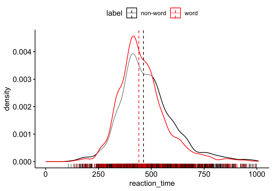
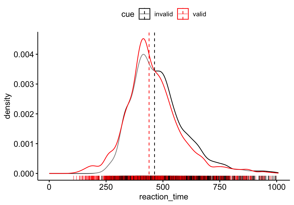
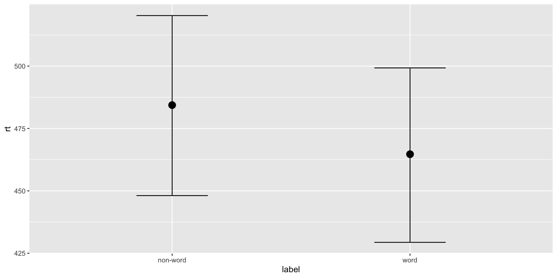
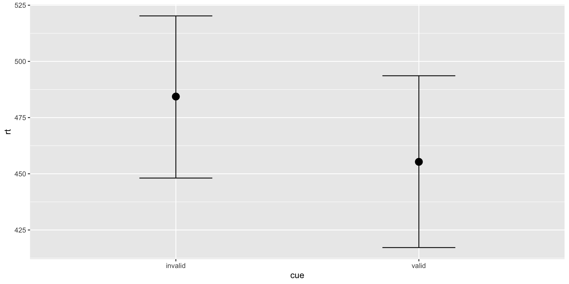
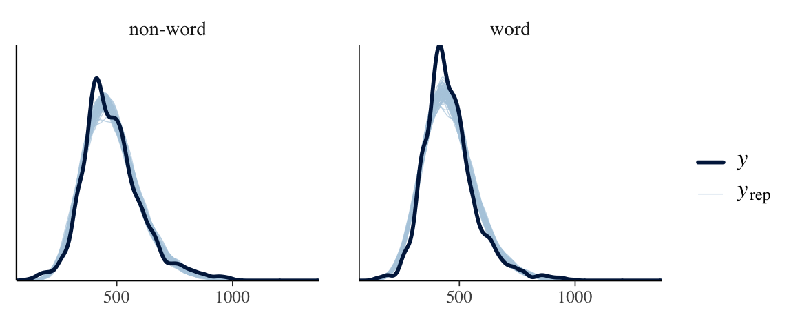
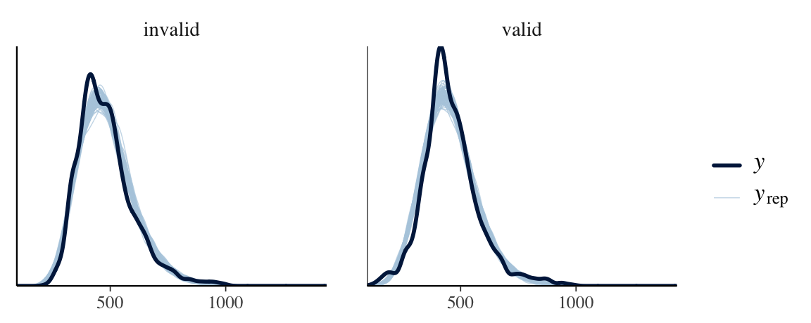
Experiment: participants viewed a central prime—either a real word or pseudo-word—followed by a spatial cue directing them to a target on the left or right, which they located by pressing a key.