Reproducible Science

Methodological School - 3 R’s of Trustworthy Science

Margherita Calderan

May 18, 2026

About me :)

• Post-doctoral researcher, University of Padova.
• Research: Bayesian hypothesis testing, computational modeling of cognitive and learning processes.
• Passion: Soccer and Reproducible science, driven by early struggles with messy datasets and a belief in transparent research!

That’s why I’m here today: to talk about reproducible science as a concrete way to improve the quality and transparency of our research.

Our job is hard

• Running experiments

• Analyzing data

• Managing trainees

• Writing papers

• Responding to reviewers
  

It’s a lot. It’s easy to feel overwhelmed. And in that chaos, good practices often fall by the wayside. It’s tempting to write quick scripts, save datasets with unclear names, copy and paste plots into Word, and move on. But here’s the thing: all of those shortcuts come at a cost.

Reproducibility helps!

• Organizes your workflow.

• Saves time by documenting steps.

• Builds trust in your findings.

• Enables others to reproduce and extend your work.

I want to suggest that reproducibility is not an extra task. It’s not a burden we add on top of everything else. It’s a way of working that can replace the mess with a clear system. It’s an investment in your future self.

What is reproducible science?

Reproducibility can be considered as the most fundamental pre-requisite of replication in science.

“…obtaining consistent results using the same input data, computational steps, methods, and code, and conditions of analysis.” Reproducibility et al. (2019)

Meaning that someone else, or even you, in the future, can reproduce your results from your materials: your data, your code, your documentation.

The experimental design, data and methodologies of analysis are all fixed. A reproducible research paper should provide enough information to obtain the results originally reported, starting from the same raw data. Raw data are data in a form as close as possible to what was generated by the original experimental source.

Keys to reproducible science

• Data: organize, document, and share your datasets in ways that are usable by others and understandable by you (even years later).
• Code: write analysis scripts that are clean, transparent, and reusable.
• Literate programming: combine code and text in the same document, so your reports are dynamic and replicable.
• Version Control and Sharing: track changes, collaborate, and make your work openly available using tools like GitHub and OSF (and/or Zenodo).

We need to organize, document, and share our data so it’s clear to others. Our analysis code should be clean, transparent, and reusable. By combining code and text in the same document, we make our work dynamic and understandable. And with version control tools like Git, we can track changes, collaborate, and share our work openly.

So… Is reproducible science even harder?

Learning takes effort. It can feel slow and confusing. But once you’ve learned these tools, your workflow becomes smoother.

Outline

1. Data

2. Code

3. R projects

4. Literate Programming

5. Version Control

In the sections that follow, we’ll explore how to: • Document and structure your data, • Write readable, testable code, • Use functional programming principles to simplify your workflow, • Organize your projects in a way that’s portable and consistent, • And write scientific documents that are both human-readable and machine-executable.

Data

If your data is messy, undocumented, or inaccessible, it doesn’t matter how brilliant your analysis is, no one will be able to follow it, reproduce it, or extend it.

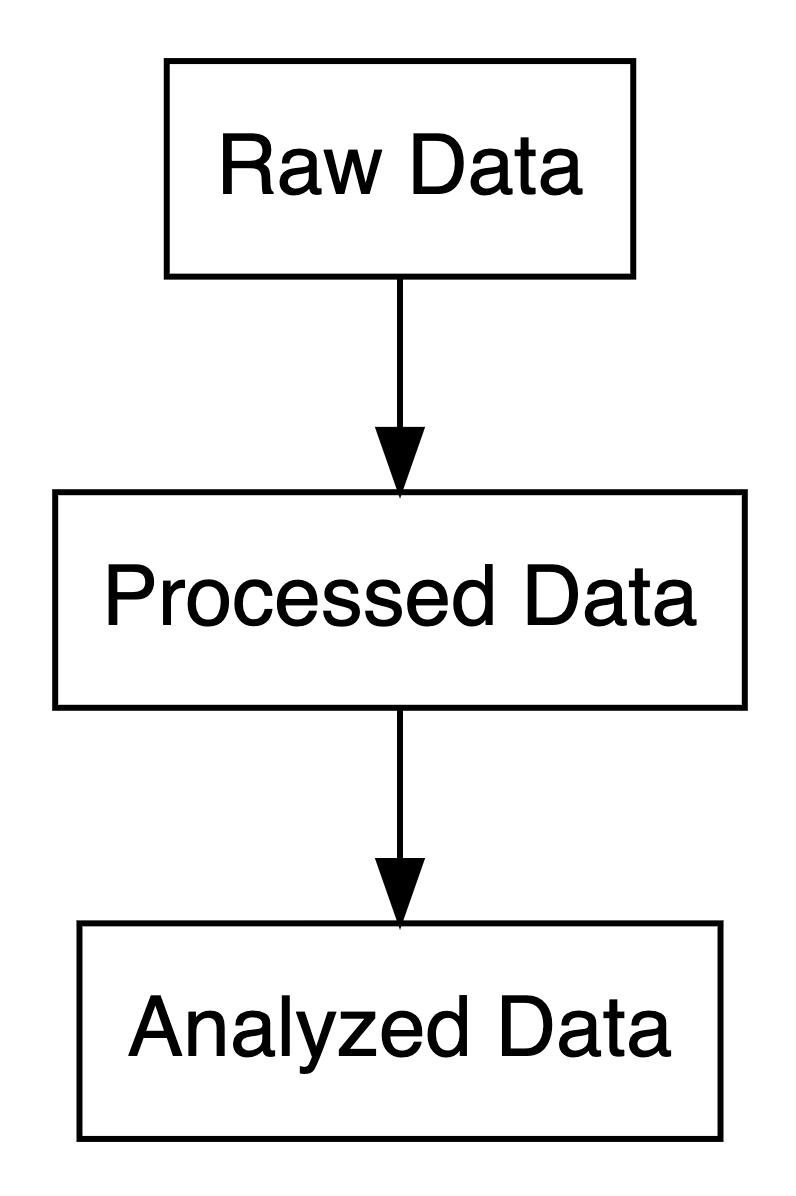
Data types in research

• Raw Data: Original, unprocessed (e.g., survey responses).
• Processed Data: Cleaned, digitized, or compressed.
• Analyzed Data: Summarized in tables, charts, or text.

Share all your data: where?

• dryad

• zenodo

• osf

Why use dryad?

• Flexible: Accepts any file format from any field.

• Citable: Provides a persistent DOI.

• Curated: Data curators check files for best practices.

• Integrated: Streamlines sharing with publishers (Wiley, Royal Society, PLOS).

Why use zenodo?

• Secure: Stored safely in CERN’s Data Centre.

• Citable: Every upload gets a DOI.

• Controlled Access: Can restrict access for sensitive data (e.g., clinical trials).

• GitHub Integration: Easily preserve your GitHub repositories.

Why use osf?

• Collaborative: Add collaborators and manage projects

• Citable: Every file gets a unique URL for citing, project gets a DOI.

• Comprehensive: Automate version control, preregister research, and share preprints.

• Long-term: Guaranteed 50+ years of read access hosting

• GitHub Integration: Easily preserve your GitHub repositories.

Bad data sharing example

Imagine this scenario: you read a paper that seems really relevant to your research. At the end, you’re excited to see they’ve shared their data on OSF. You go to the repository, and there’s one file…

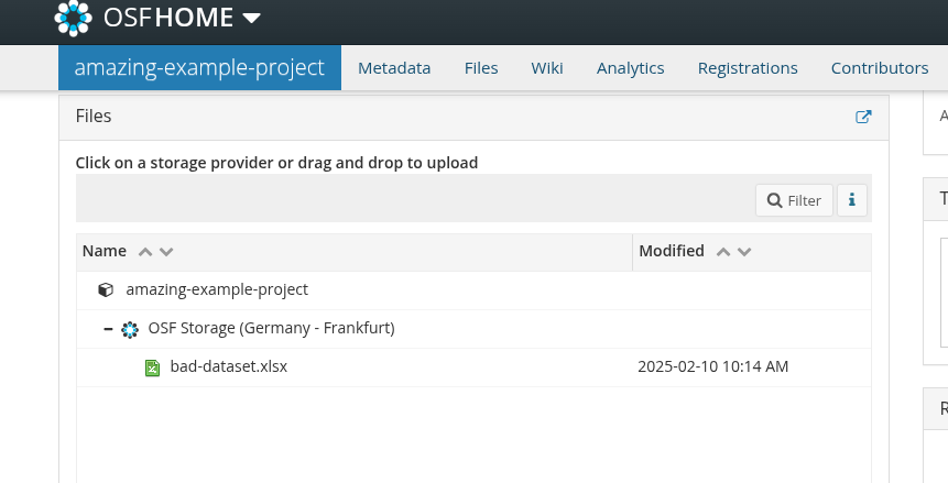
Bad data sharing example

You download it, open it, and you see this…

x1	x2	x3	x4	x5	x6	x7
0.3981105	13.912435	a	0	-0.6775811	0.8759740	-0.2051604
-0.1434733	1.093743	c	0	0.7055193	0.2521987	1.8816947
-0.2526000	4.898035	c	0	0.4744651	-0.5628840	0.3245589
-1.2272588	14.717053	b	0	-0.5132792	-1.1368242	-0.1355150
-0.4360417	8.547025	c	1	-0.1736804	-0.7120962	-1.2714320

What do these variables mean? What’s x3?

What do 0 and 1 represent?

How are missing values coded?

Is x6 a z-score or raw data?

There’s no README file. No codebook. No context. Even though this file is technically shared, it’s not reproducible. It’s not even interpretable. And again, this is assuming we’re lucky and the file opens properly.

Good data sharing practices

• Use plain-text formats (e.g., .csv, .txt).
• Include a data dictionary with variable descriptions.
• Add a README with key details.
• Follow FAIR principles (Findable, Accessible, Interoperable, Reusable; Wilkinson et al. (2016), https://www.go-fair.org/fair-principles/)

They’re easy to read, easy to import- Avoid Excel files or other proprietary formats that often create compatibility issues. Plain text is portable. It doesn’t care what operating system or software someone uses.

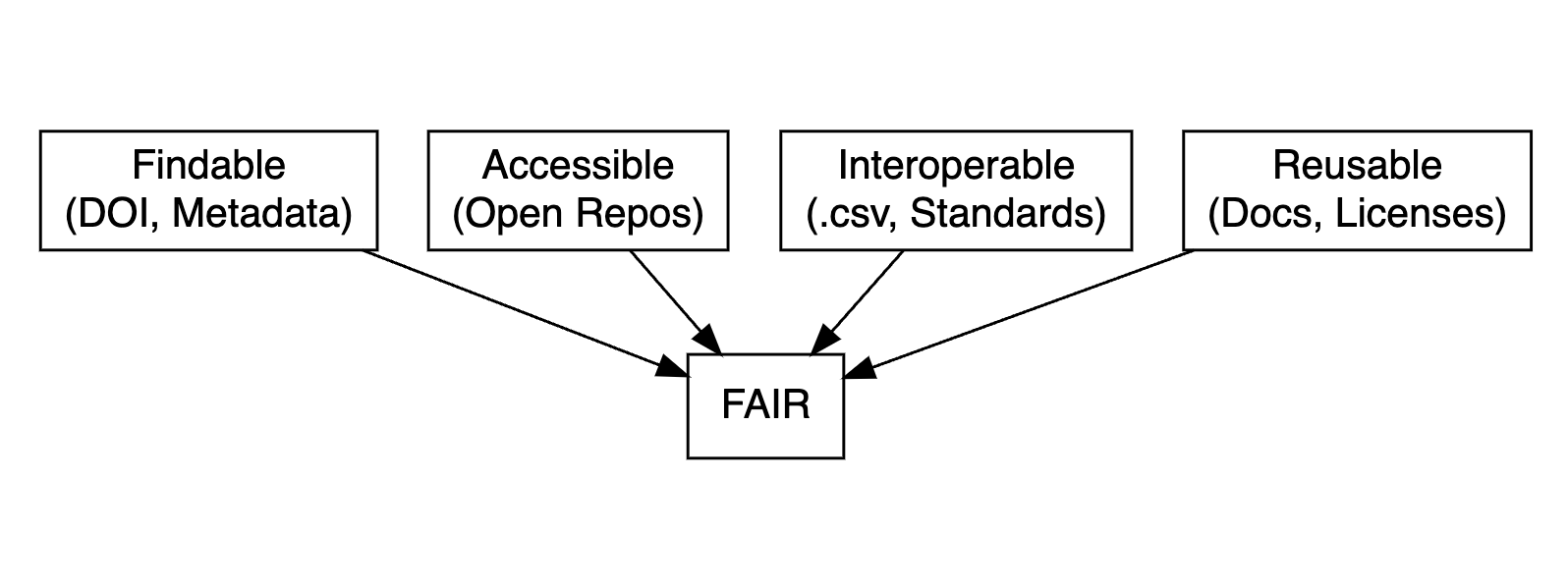
FAIR data principles

• Findable: Use metadata and DOIs to make data easy to locate.
• Accessible: Ensure data is retrievable via open repositories.
• Interoperable: Use standard formats (e.g., .csv, .txt) for compatibility.
• Reusable: Include clear documentation and open licenses.

Your data should be discoverable. That means metadata, proper naming, and a DOI if possible. Others should be able to download your data, ideally without jumping through hoops. Use standard formats and vocabulary so that your data can be combined with other datasets. Provide enough documentation and licensing that others can actually reuse your data appropriately.

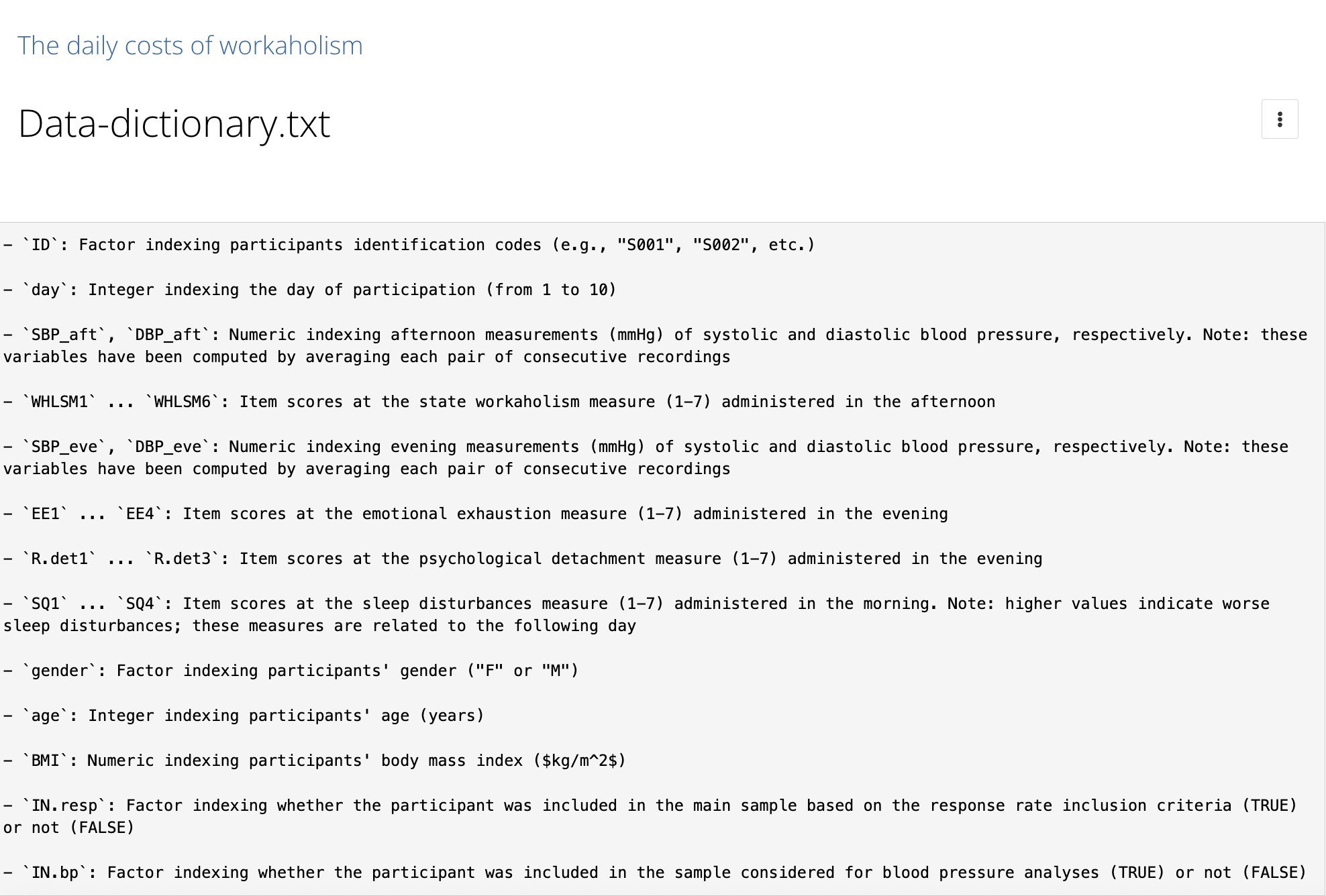
Data dictionary

A data dictionary is a document that outlines the structure, content, and variable definitions for a dataset (harvard/datamanagement).

It is critical for reproducibility because it explains what all the variable names and values in your spreadsheet really mean (osf/datadictionary).

Data dictionary

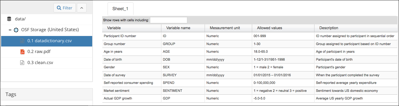
From OSF guide

• Variable names
• Human-readable variable names
• Measurement units for the variable
• Allowed values for the variable
• Definition of the variable

if a column contains measurements of time, it should be clear whether they are measured in hours, minutes, or seconds. Allowed values A column should contain the range of values or accepted values for the variable. This helps identify data entry errors.

Data dictionary: let’s try

Imagine we are collecting data (n = 12) to explore the relationship between anxiety (measured via the State-Trait Anxiety Inventory) and education levels:

(df <- data.frame(id = factor(paste(letters[1:12], rbinom(12, 12, 0.5), sep = "")), 
                 anxi = rpois(12, 50),
                 edu = factor(rep(c("PhD", "BSc", "MSc"), each = 4))))

   id anxi edu
1  a6   50 PhD
2  b5   59 PhD
3  c9   37 PhD
4  d3   46 PhD
5  e7   48 BSc
6  f6   44 BSc
7  g7   56 BSc
8  h4   54 BSc
9  i6   42 MSc
10 j4   48 MSc
11 k6   48 MSc
12 l4   37 MSc

STAI-T consists of 20 items, 4-points likert scale

datadictionary

library(datadictionary)

descr <- list(
  anxi = "Anxiety symptoms measured with the State-Trait Anxiety Inventory (state scale); 20 items summed on a 4-point Likert scale.",
  edu  = "Highest degree obtained, factor with three levels: PhD, BSc, MSc")

datdi <- create_dictionary(df, id_var = "id",
                    var_labels = descr)

Data dictionary

gt::gt(datdi)

item	label	class	summary	value
			Rows in dataset	12
			Columns in dataset	3
id	Unique identifier		unique values	12
			missing	0
anxi	Anxiety symptoms measured with the State-Trait Anxiety Inventory (state scale); 20 items summed on a 4-point Likert scale.	integer	mean	47
			median	48
			min	37
			max	59
			missing	0
edu	Highest degree obtained, factor with three levels: PhD, BSc, MSc	factor	BSc (1)	4
			MSc (2)	4
			PhD (3)	4
			missing	0

Data dictionary - Good data sharing example

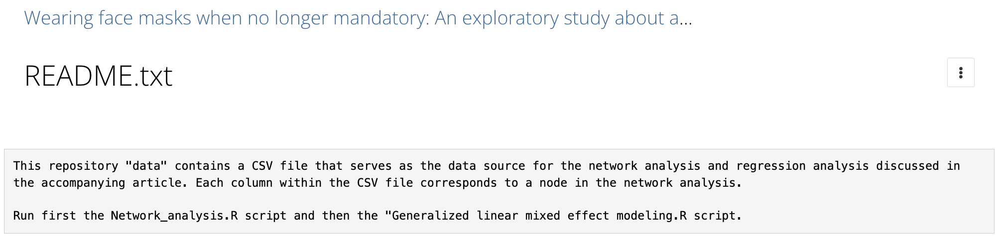
README

A README file is the first thing someone sees when they open your dataset (or project folder). It should answer basic questions like:

• What is this dataset?
• How was it collected?
• What are the variables?
• Which is the structure of the project?

Don’t overthink it, just write it like you’re explaining the dataset to a curious but uninformed colleague.

README

Anxiety and Education Example Dataset

This repository contains a small simulated dataset with 12 observations, designed to explore the relationship between anxiety and education level.

Anxiety is measured using the State-Trait Anxiety Inventory (STAI), specifically the trait scale. Education level is recorded as the highest degree obtained (Bachelor, Master, PhD).

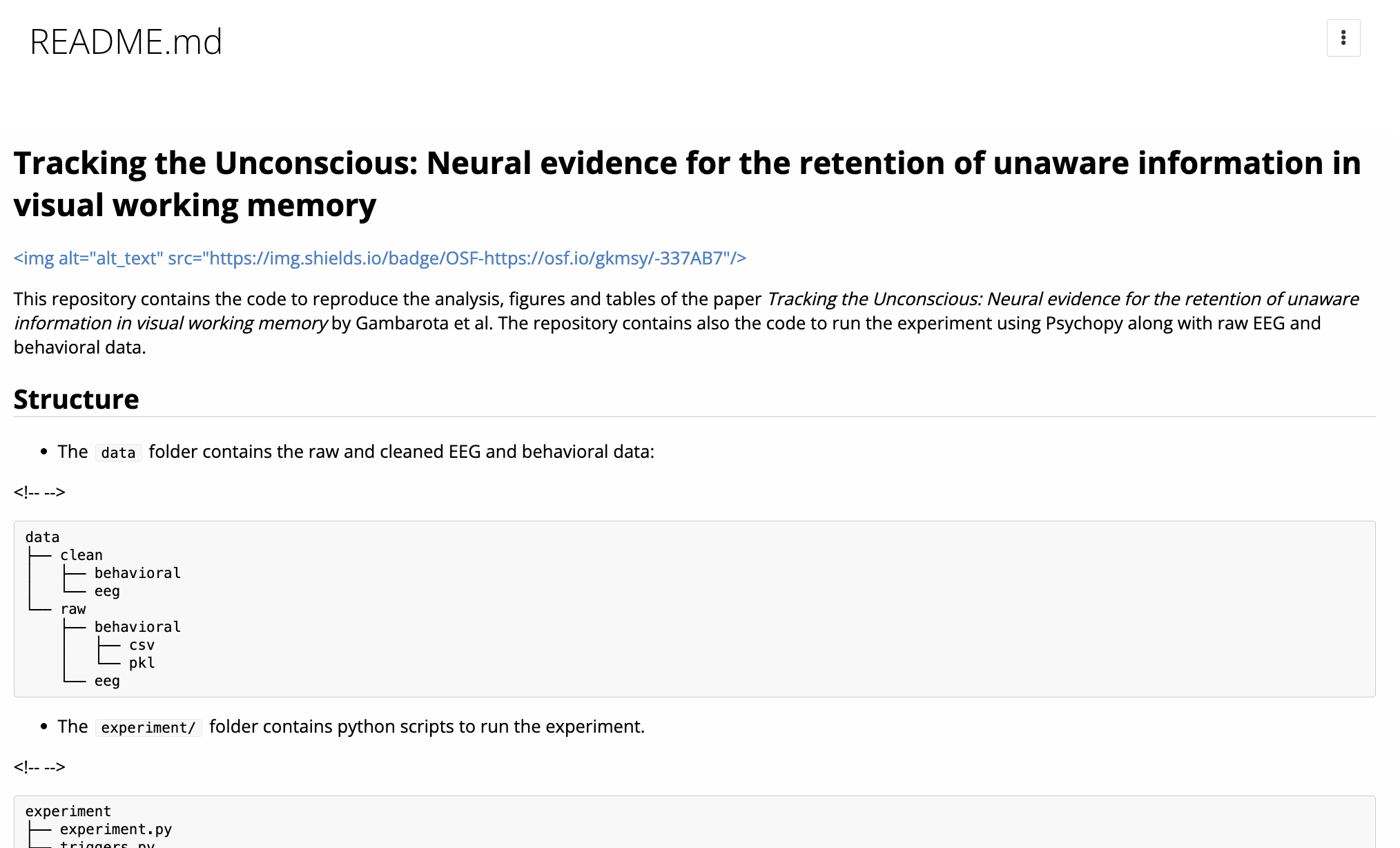
README - Good example

README - Good example

Data licensing

A license tells others what they can and can’t do with your data. If you don’t include one, legally speaking, people might not be allowed to use it, even if you meant to share it openly.

Data licensing

Common licenses for documents, data, and other non‑software:

• CC BY: Permits reuse of documents, data, and other non‑software works with attribution.

• CC0: Places documents, data, or other works in the public domain; no restrictions on reuse.

Data licensing

Common licenses for software:

• GNU GPL‑3.0: Applies to software and guarantees freedom to run, study, share, and modify software, requiring modified versions be distributed under the same license.

• AGPL‑3.0: Extends the GNU GPL by requiring source code to be made available if a modified version runs on a publicly accessible server.

Exercise: Prepare your data‑sharing package

Before collecting data, good practice is to plan how you will document and share it.

Imagine you are designing the following study:

A research team wants to investigate whether daily screen time is associated with sleep quality in university students. They plan to recruit 200 participants and collect the following variables: average daily screen time, sleep duration, and age.

Your tasks:

1. Data dictionary: you can use a .csv, Excel file, R or create a table in word.
2. README: write a short text.
3. License: choose a license for the dataset and justify your choice.

Code

Now that we’ve talked about how to document and organize your data, let’s move to the next part : your code. Just like with data, your code can either be a gateway to understanding, or a brick wall. And unfortunately, many of us learn to code the way we learn to cook when we’re hungry: quickly, messily, and without a recipe. That might work in the moment, but if someone else, like your collaborator or your reviewer tries to understand what you did… it’s going to be tough. So let’s talk about how to write clear, organized, and reproducible code.

Why scripting?

SPSS workflow:

• Click menu items to run analysis

• “exclude <18”

• Click through everything again

• Forget a step? Round differently?

Stressful, error-prone, and undocumented.

Why scripting?

R workflow:

# Load data
data <- read.csv("data.csv")

# Filter age
data <- data[data$age >= 18, ]

# Analyze
summary(lm(score ~ condition, data = data))

# Make plot
ggplot(data, aes(x = condition, y = score)) +
  geom_boxplot()

One line change, rerun, and everything updates.

You go into your code, change one line: filter(age >= 18), and rerun everything. The tables update, the figures update, the results update, and you’re done. No mistakes, no stress, and your analysis is documented.

Why scripting?

Scripting ensures transparent and reproducible workflows.

Reproducible: You can rerun them.

Documented: You can see what you did and when.

Shareable: Others can inspect and reproduce your analysis.

they’re debuggable. If something goes wrong, you can trace it.

and RStudio

• R: Free, open-source, with thousands of packages for analysis.
• RStudio: Intuitive interface for coding, plotting, and debugging.
• Vibrant community for support and resources.

Writing better code

• Name descriptively: Use snake_case or camelCase for readability.
• Comment clearly: Document your logic for clarity.
• Organize scripts: Load packages and data upfront.

Use descriptive names

# Bad 
x1 <- c("UNIPD psychology", "university of padova medicine", "unito_biology")


# Better
uniDep <- c("unipdPsy", "unipdMed", "unitoBio")

Comments, comments and comments…

Write the code for your future self and for others, not for yourself right now.

study_final <- study_raw |>
  
  # 1. Focus on participants who completed the primary outcome
  filter(!is.na(anxiety_score)) |>
  
  # 2. Convert raw scores to clinical categories
  mutate(severity = if_else(anxiety_score > 15, "High", "Low")) |>
  
  # 3. Drop pilot-phase data (pre-2024)
  filter(date >= as.Date("2024-01-01")) 

Try to open a (not well documented) old code after a couple of years and you will understand :)

Let’s be honest: we all think we’ll remember what we did. We never do. That’s why comments are essential. They don’t have to be elaborate, but they should describe why you’re doing something, especially if it’s not obvious.

Organized scripts

Global operations at the beginning of the script:

• loading packages
• changing general options (options())
• loading datasets

# load packages
library(tidyverse) # manipulation
library(ggplot2) # graphic

# options
options(scipen = 999) # digits
set_theme(theme_classic(base_size = 16)) # theme for plots

# load data
dat <- read.csv(...)

It’s readable. It’s linear. And if something breaks, you know where to look.

Functions to avoid repetition

Functions are the primary building blocks of your program. You write small, reusable, self-contained functions that do one thing well, and then you combine them.

Avoid repeating the same operation multiple times in the script. The rule is, if you are doing the same operation more than two times, write a function.

A function can be re-used, tested and changed just one time affecting the whole project.

If you’ve ever found yourself writing the same line of code over and over again, copying and pasting blocks of logic for different variables, or modifying dozens of lines when one thing change. It’s a way to write clearer, shorter, and less error-prone code.

Functional programming, example…

We have a dataset (mtcars) and we want to calculate the mean, median, standard deviation, minimum and maximum of each column and store the result in a table.

head(mtcars, n = 3) # display first 3 rows

               mpg cyl disp  hp drat    wt  qsec vs am gear carb
Mazda RX4     21.0   6  160 110 3.90 2.620 16.46  0  1    4    4
Mazda RX4 Wag 21.0   6  160 110 3.90 2.875 17.02  0  1    4    4
Datsun 710    22.8   4  108  93 3.85 2.320 18.61  1  1    4    1

str(mtcars) # show structure

'data.frame':   32 obs. of  11 variables:
 $ mpg : num  21 21 22.8 21.4 18.7 18.1 14.3 24.4 22.8 19.2 ...
 $ cyl : num  6 6 4 6 8 6 8 4 4 6 ...
 $ disp: num  160 160 108 258 360 ...
 $ hp  : num  110 110 93 110 175 105 245 62 95 123 ...
 $ drat: num  3.9 3.9 3.85 3.08 3.15 2.76 3.21 3.69 3.92 3.92 ...
 $ wt  : num  2.62 2.88 2.32 3.21 3.44 ...
 $ qsec: num  16.5 17 18.6 19.4 17 ...
 $ vs  : num  0 0 1 1 0 1 0 1 1 1 ...
 $ am  : num  1 1 1 0 0 0 0 0 0 0 ...
 $ gear: num  4 4 4 3 3 3 3 4 4 4 ...
 $ carb: num  4 4 1 1 2 1 4 2 2 4 ...

Imperative programming

The standard (~imperative) option is using a for loop, iterating through columns, calculate the values and store into another data structure.

ncols <- ncol(mtcars) # number of columns
# create vectors of length ncols with 0s
means <- medians <- mins <- maxs <- rep(0, ncols)

# loop over the columns (variables) and fill the vectors
for(i in 1:ncols){
  means[i] <- mean(mtcars[[i]])
  medians[i] <- median(mtcars[[i]])
  mins[i] <- min(mtcars[[i]])
  maxs[i] <- max(mtcars[[i]])
}

# combine everything into a df
results <- data.frame(means, medians, mins, maxs)
results$col <- names(mtcars) # add variable names

head(results, n = 3) # display 3 rows

      means medians mins  maxs  col
1  20.09062    19.2 10.4  33.9  mpg
2   6.18750     6.0  4.0   8.0  cyl
3 230.72188   196.3 71.1 472.0 disp

Functional programming

The main idea is to decompose the problem writing a function and loop over the columns of the dataframe:

summ <- function(x){
  data.frame(means = mean(x), #given an input compute stats
             medians = median(x), 
             mins = min(x), 
             maxs = max(x))
} # return a df

ncols <- ncol(mtcars) #number of columns
dfs <- vector(mode = "list", length = ncols) #empty list 

for(i in 1:ncols){
  dfs[[i]] <- summ(mtcars[[i]]) 
  #each element of the list is a df with the summary stat
}

Functional programming

#combine list to obtain data.frame
results <- do.call(rbind, dfs)
results$var <- names(mtcars) # add variable names
head(results, n = 3) # display 3 rows

      means medians mins  maxs  var
1  20.09062    19.2 10.4  33.9  mpg
2   6.18750     6.0  4.0   8.0  cyl
3 230.72188   196.3 71.1 472.0 disp

Functional programming, *apply 📦

• The *apply family is one of the best tool in R. The idea is pretty simple: apply a function to each element of a list.

• The powerful side is that in R everything can be considered as a list. A vector is a list of single elements, a dataframe is a list of columns etc.

• Internally, R is still using a for loop but the verbose part (preallocation, choosing the iterator, indexing) is encapsulated into the *apply function.

means <- rep(0, ncol(mtcars))

for(i in 1:length(means)){
  means[i] <- mean(mtcars[[i]])
}

# the same with sapply
means <- sapply(mtcars, mean)

The *apply family

Apply your function…

results <- lapply(mtcars, summ) 

Now results is a list of data frames, one per column.

We can stack them into one big data frame:

results_df <- do.call(rbind, results)
head(results_df, n = 5)

          means medians  mins   maxs
mpg   20.090625  19.200 10.40  33.90
cyl    6.187500   6.000  4.00   8.00
disp 230.721875 196.300 71.10 472.00
hp   146.687500 123.000 52.00 335.00
drat   3.596563   3.695  2.76   4.93

This gives us a clean summary for every variable in just a few lines of code. No loops, no repetition.

Using sapply, vapply, and apply

• lapply() always returns a list.
• sapply() tries to simplify the result into a vector or matrix.
• vapply() is like sapply() but safer (you specify the return type).
• apply() is for applying functions over rows or columns of a matrix or data frame.

for loops are bad?

for loops are the core of each operation in R (and in every programming language). For complex operation they are more readable and effective compared to *apply. In R we need extra care for writing efficent for loops.

Extremely slow, no preallocation:

res <- c()
for(i in 1:1000){
  # do something
  res[i] <- i^2
}

Very fast:

res <- rep(0, 1000)
for(i in 1:length(res)){
  # do something
  res[i] <- i^2
}

microbenchmark 📦

library(microbenchmark)

microbenchmark(
  grow_in_loop = {
    res <- c()
    for (i in 1:10000) {
      res[i] <- i^2  
    }
  },
  preallocated = {
    res <- rep(0, 10000)
    for (i in 1:length(res)) {
      res[i] <- i^2  
    }
  }, times = 100)[1:2,1:2]

Unit: microseconds
         expr      min       lq     mean   median       uq      max neval
 grow_in_loop 1271.656 1271.656 1271.656 1271.656 1271.656 1271.656     1
 preallocated  884.329  884.329  884.329  884.329  884.329  884.329     1

Going further: custom function lists

Let’s define a list of functions:

funs <- list(mean = mean, sd = sd, 
             min = min, max = max, median = median)

Now we can apply all of these to every column:

# MARGIN = 2 = column
sapply(funs, function(f) apply(mtcars, MARGIN = 2, f)) 

           mean          sd    min     max  median
mpg   20.090625   6.0269481 10.400  33.900  19.200
cyl    6.187500   1.7859216  4.000   8.000   6.000
disp 230.721875 123.9386938 71.100 472.000 196.300
hp   146.687500  68.5628685 52.000 335.000 123.000
drat   3.596563   0.5346787  2.760   4.930   3.695
wt     3.217250   0.9784574  1.513   5.424   3.325
qsec  17.848750   1.7869432 14.500  22.900  17.710
vs     0.437500   0.5040161  0.000   1.000   0.000
am     0.406250   0.4989909  0.000   1.000   0.000
gear   3.687500   0.7378041  3.000   5.000   4.000
carb   2.812500   1.6152000  1.000   8.000   2.000

This gives you a matrix with rows as variables and columns as statistics.

Test your functions - fuzzr 📦

When you write your own functions, it’s smart to test them. In R, we can use fuzzr to do property-based testing.

Define your function…

my_mean <- function(x, na.rm = TRUE) {
  if (!is.numeric(x)) stop("`x` must be numeric")
  if (length(x) == 0) return(NA)
  if (na.rm) x <- x[!is.na(x)]
  if (length(x) == 0) return(NA)
  sum(x) / length(x)
}

Define properties that should always hold true…

property_mean_correct <- function(x) {
  x_no_na <- x[!is.na(x)] #remove NA
  if (length(x_no_na) == 0) return(TRUE)
  abs(my_mean(x) - mean(x, na.rm = TRUE)) < 1e-8
}

This runs the property on different random numeric vectors and checks whether it holds.

# Property-based testing with 'fuzzr'
library(fuzzr)
test = fuzz_function(fun = property_mean_correct, 
                     arg_name = "x", 
                     tests = test_dbl()) 
lapply(test, function(res) res$test_result$value)

[[1]]
[1] TRUE

[[2]]
[1] TRUE

[[3]]
[1] TRUE

[[4]]
[1] TRUE

[[5]]
[1] TRUE

[[6]]
[1] TRUE

fuzzr::test_dbl()

$dbl_empty
numeric(0)

$dbl_single
[1] 1.5

$dbl_mutliple
[1] 1.5 2.5 3.5

$dbl_with_na
[1] 1.5 2.5  NA

$dbl_single_na
[1] NA

$dbl_all_na
[1] NA NA NA

Why functional programming?

• We can write less and reusable code that can be shared and used in multiple projects.

• The scripts are more compact, easy to modify and less error prone (imagine that you want to improve the summ function, you only need to change it once instead of touching the for loop).

• Functions can be easily and consistently documented (see roxygen documentation) improving the reproducibility and readability of your code.

Import your functions

You can write some R scripts only with functions and source() them into the global environment.

project/
│
├─ R/
│  │
│  ├─ utils.R
   │
   ├─ analysis.R
   
   

source("R/utils.R")
results <- lapply(mtcars, summ)
results_df <- do.call(rbind, results)

More about functional programming in R

• Advanced R by Hadley Wickham, section on Functional Programming (https://adv-r.hadley.nz/fp.html)

• Hands-On Programming with R by Garrett Grolemund https://rstudio-education.github.io/hopr/

• Hadley Wickham: The Joy of Functional Programming (for Data Science)(https://www.youtube.com/watch?v=bzUmK0Y07ck)

Wrapping up

• Avoid repetition by using functions.
• Test your functions.
• The *apply functions are your friends, or *map from purrr 📦

In the long run, these practices will save you time, reduce your bugs, and make your research far easier to reproduce.

Organize your project

How do we keep everything together, our data, our scripts, our figures, our notes, in a way that is coherent, portable, and reproducible?

R Projects

R Projects are a feature implemented in RStudio to organize a working directory.

• They automatically set the working directory
• They allow the use of relative paths instead of absolute paths
• They provide quick access to a specific project

The working directory problem

How many times have you opened an R script and seen this at the top?

setwd("C:/Users/margherita/Documents/PhD/final_data/") #change

Instead of hardcoding paths, we want to use projects with relative paths.

This works perfectly on one computer. But the moment someone else tries to run it, or even you open it from a different machine or folder, it breaks.

R Projects

An R Project (.Rproj) is a file that defines a self-contained workspace.

When you open an R Project, your working directory is automatically set to the project root, no need to use setwd() ever again.

Open RStudio

File → New Project → New Directory → New Project

Relative Path (to the working directory)

Users
 |
 ├─tita
    |
    ├─ sleep-memo
           |
           ├─ data
           |    ├─ raw.csv
           |
           ├─ sleep-memo.Rproj

Absolute path:

read.csv("Users/tita/sleep-memo/data/raw.csv") 

Relative path:

read.csv("data/raw.csv")

This makes your code portable. Anyone can clone your project and run it from their own computer, and the paths will still work.

A minimal project structure

  my-project/
      │
      ├── data/
      │     ├── raw/
      │     └── processed/
      ├── R/
      │   └── analysis.R
      │ 
      ├── outputs/
      │   ├── figures/
      │   └── tables/
      │
      ├── my-project.Rproj
      │
      └── README.md

This isn’t rigid, you can adapt it. But the key idea is: one folder, one project, everything in its place.

Project organization with rrtools 📦

To make this even “easier”, you can use the rrtools package to create what’s called a reproducible research compendium.

… the goal is to provide a standard and easily recognisable way for organising the digital materials of a project to enable others to inspect, reproduce, and extend the research… (Marwick, Boettiger, and Mullen 2018)

Research compendium rrtools 📦

• Organize its files according to the prevailing conventions.
• Maintain a clear separation of data (original data is untouched!), method, and output.
• Specify the computational environment that was used for the original analysis

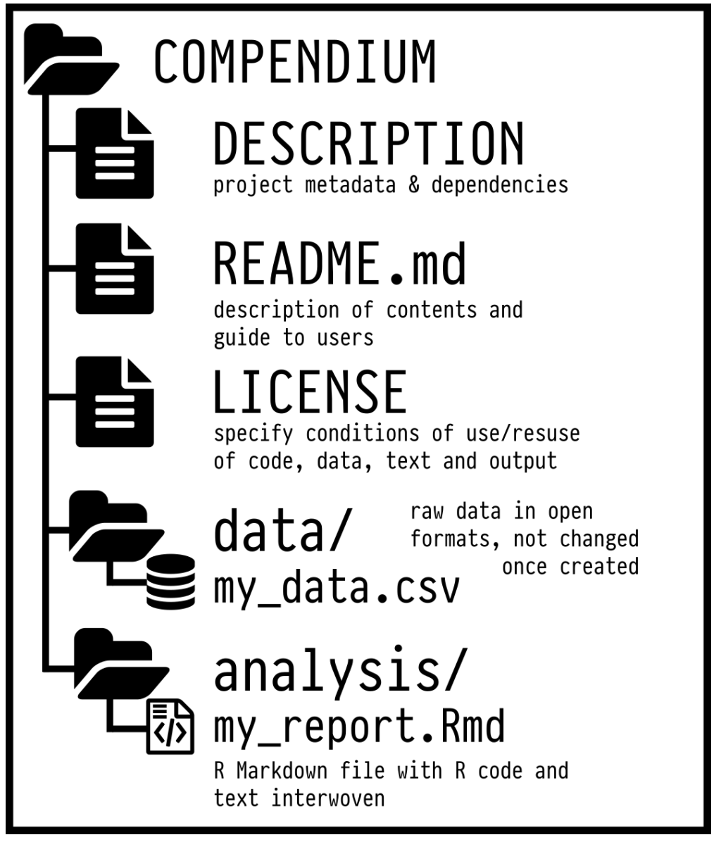
rrtools::create_compendium("compedium") builds the basic structure for a research compendium.

> Example

> Tutorial

These features enable managing, installing, and sharing project-related functionality.

renv📦 : locking your R environment

Another challenge for reproducibility is package versions.

You write some code today using dplyr 1.1.2.

In six months, dplyr gets updated… 😢

renv helps you create reproducible environments for your R projects!

What does renv do?

• It records all the packages you use, with versions, in a lockfile

• It installs them in a project-specific library

• It ensures that anyone who runs your code gets exactly the same environment

Project specific library

install.packages("renv")

renv::init()

install.packages('bayesplot')

# These packages will be installed into 
# "~/repro-pre-school/example-renv/renv/library/macos/R-4.4/aarch64-ap# ple-darwin20".

> Example

renv commands

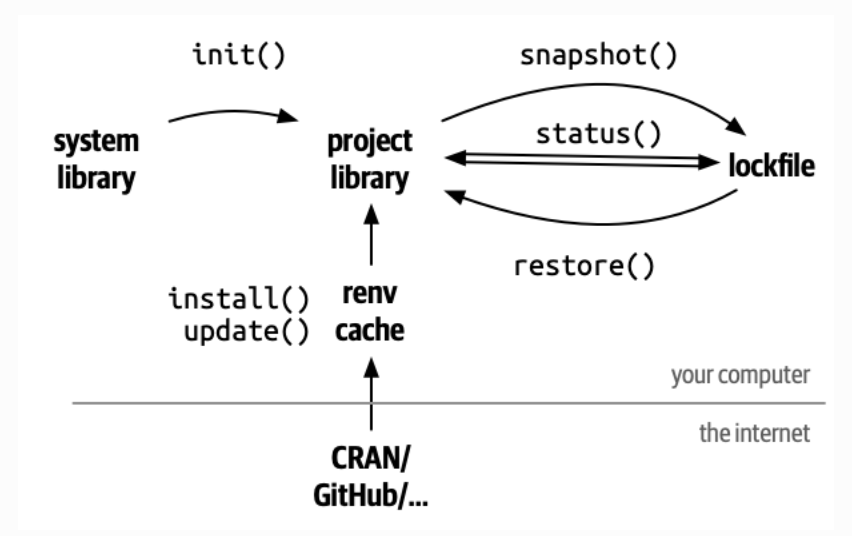
renv::restore() # re-install from lockfile

Research rrtools + renv 💣

• rrtools: Organizes your project into a reproducible compendium with clear folders.
• renv: Locks R package versions for consistent environments.
• Together, they ensure structure and reproducibility across teams and time.
• Run rrtools::create_compendium("project") to start, then renv::init() to lock dependencies.

Docker

• Packages your project’s software, dependencies, and system settings into a container.
• Ensures consistency across different computers or servers.
• Ideal for sharing complex analyses with others.

Documenting your environment ℹ️

• sessionInfo(): Captures your R version, packages, and platform in one command.
• Easy way to document and share your environment.

sessionInfo()

R version 4.4.2 (2024-10-31)
Platform: aarch64-apple-darwin20
Running under: macOS Sequoia 15.6.1

Matrix products: default
BLAS:   /Library/Frameworks/R.framework/Versions/4.4-arm64/Resources/lib/libRblas.0.dylib 
LAPACK: /Library/Frameworks/R.framework/Versions/4.4-arm64/Resources/lib/libRlapack.dylib;  LAPACK version 3.12.0

locale:
[1] en_US.UTF-8/en_US.UTF-8/en_US.UTF-8/C/en_US.UTF-8/en_US.UTF-8

time zone: Europe/Rome
tzcode source: internal

attached base packages:
[1] stats     graphics  grDevices utils     datasets  methods   base     

other attached packages:
[1] fuzzr_0.2.2          microbenchmark_1.5.0 datadictionary_1.0.1
[4] patchwork_1.3.2      ggplot2_4.0.2       

loaded via a namespace (and not attached):
 [1] gt_1.0.0           sandwich_3.1-1     tidyr_1.3.2        sass_0.4.10       
 [5] generics_0.1.4     xml2_1.3.8         stringi_1.8.7      lattice_0.22-6    
 [9] hms_1.1.4          digest_0.6.39      magrittr_2.0.4     evaluate_1.0.5    
[13] grid_4.4.2         timechange_0.4.0   RColorBrewer_1.1-3 mvtnorm_1.3-3     
[17] fastmap_1.2.0      cellranger_1.1.0   jsonlite_2.0.0     Matrix_1.7-2      
[21] zip_2.3.3          survival_3.8-3     multcomp_1.4-29    mgcv_1.9-1        
[25] purrr_1.2.1        scales_1.4.0       TH.data_1.1-3      codetools_0.2-20  
[29] cli_3.6.5          labelled_2.16.0    rlang_1.1.7        splines_4.4.2     
[33] withr_3.0.2        yaml_2.3.12        otel_0.2.0         tools_4.4.2       
[37] dplyr_1.2.0        forcats_1.0.1      assertthat_0.2.1   vctrs_0.7.1       
[41] R6_2.6.1           zoo_1.8-12         lifecycle_1.0.5    lubridate_1.9.5   
[45] MASS_7.3-64        pkgconfig_2.0.3    pillar_1.11.1      openxlsx_4.2.8    
[49] gtable_0.3.6       glue_1.8.0         Rcpp_1.1.1         haven_2.5.4       
[53] xfun_0.56          tibble_3.3.1       tidyselect_1.2.1   rstudioapi_0.18.0 
[57] knitr_1.51.2       farver_2.1.2       htmltools_0.5.9    nlme_3.1-167      
[61] rmarkdown_2.30     labeling_0.4.3     compiler_4.4.2     S7_0.2.1          
[65] chron_2.3-62       readxl_1.4.3      

Organizing for reproducibility

• Don’t hardcode paths, use R Projects
• Create a logical folder structure for your project
• Use rrtools to scaffold a research compendium
• Use renv to lock your package versions

Literate Programming

What if your paper and your code could all live in the same file? No more copy-pasting tables from R to Word.

What’s wrong about Microsoft Word?

In MS Word (or similar) we need to produce everything outside and then manually put figures and tables.

• writing math formulas
• reporting statistics in the text
• producing tables
• producing plots

Think about the typical MW workflow

• You run your analysis in R
• You copy the results into a Word document
• You tweak the formatting
• You insert a figure generated with R manually
• You change your analysis, but forget to update the results in the text…

It’s easy to make mistakes. Your document and your data are out of sync. And your work is not reproducible.

Literate Programming

A document where:

• The code is part of the text
• The results are generated dynamically
• The figures are rendered automatically
• Everything is in sync

For example jupyter notebooks, R Markdown and now Quarto are literate programming frameworks to integrate code and text.

Literate Programming, the markup language

The markup language is the core element of a literate programming framework. When you write in a markup language, you’re writing plain text while also giving instructions for how to generate the final result.

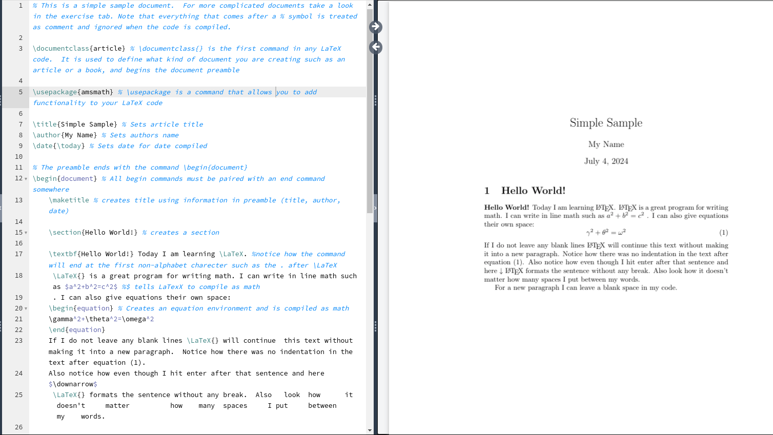
• LaTeX
• HTML
• Markdown
• …

LaTeX

Markdown

Markdown

Markdown is one of the most popular markup languages for several reasons:

• easy to write and read compared to Latex and HTML
• easy to convert from Markdown to basically every other format using pandoc

Quarto

Quarto (https://quarto.org/) is the evolution of R Markdown that integrate a programming language with the Markdown markup language. It is very simple but quite powerful.

Basic Markdown

Markdown can be learned in minutes. You can go to the following link https://quarto.org/docs/authoring/markdown-basics.html and try to understand the syntax.

Quarto

You write your documents in Markdown, and Quarto turns them into:

• HTML reports
• PDF articles
• Word documents
• Slides
• Website
• Academic manuscripts
• …

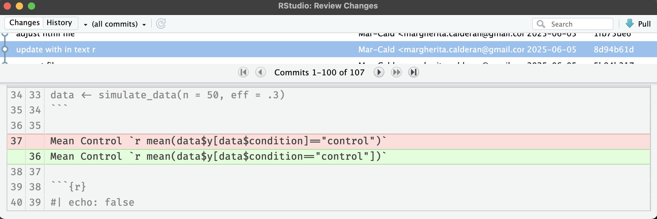
Quarto

> Example

• If your data changes, your summary table updates.
• If you update your model, your coefficients update.
• If you change a plot’s colors, the new version appear, without having to re-export and re-insert anything.

This eliminates a huge source of human error: manual updates.

Outputs

Quarto can generate multiple output formats from the same source file.

• A PDF to send to your colleagues
• A Word document for your co-author who hates PDFs
• An HTML report for your own website

Everything from the same source. No duplication. Synchronization.

> Example

Extra Tools: citations and cross-referencing

• Citations with BibTeX or Zotero
• Cross-references for figures and tables
• Numbered equations with LaTeX syntax
• Footnotes, tables of contents, and more

You can write scientific documents that look and behave just like journal articles, without ever opening Word.

Writing Papers - APA quarto

APA Quarto is a Quarto extension that makes it easy to write documents in APA 7th edition style, with automatic formatting for title pages, headings, citations, references, tables, and figures.

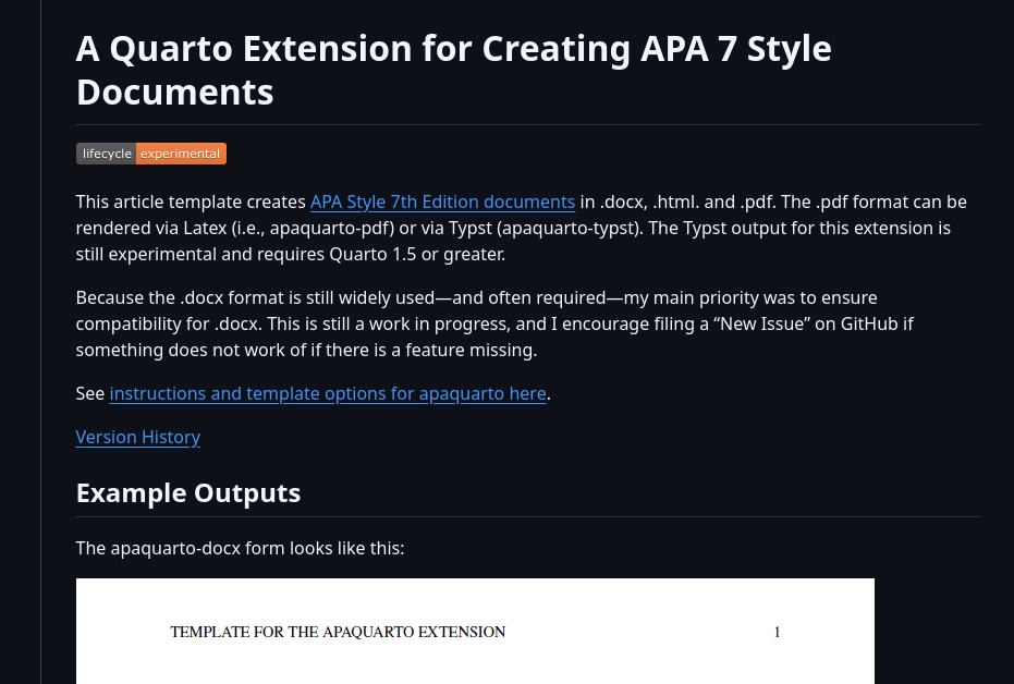
Let’s see an example…

> Example

Quarto + Zotero

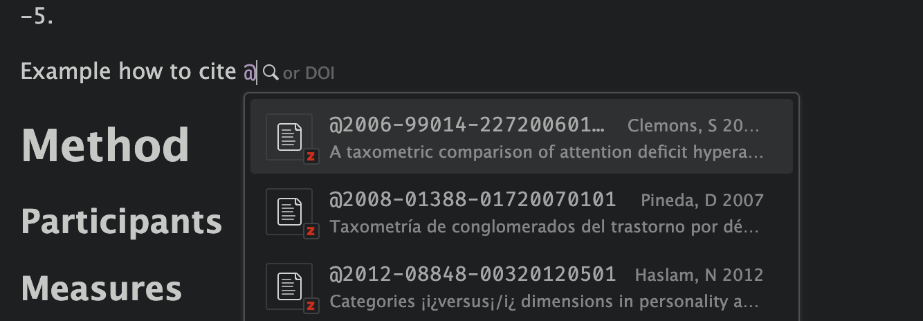
Choose your reference: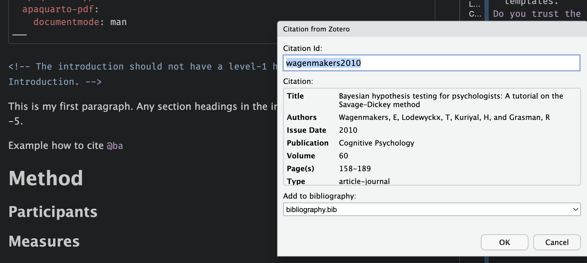

More about Quarto and R Markdown

The topic is extremely vast. You can do everything in Quarto, a website, thesis, your CV, etc.

• Yihui Xie - R Markdown Cookbook https://bookdown.org/yihui/rmarkdown-cookbook/
• Yihui Xie - R Markdown: The Definitive Guide https://bookdown.org/yihui/rmarkdown/
• Quarto documentation https://quarto.org/docs/guide/

Version Control

Why version control?

You’re working on a project. You save your script as:

• analysis.R
• analysis2.R
• analysis_final.R
• analysis_final_revised.R
• analysis_final_revised_OK_for_real.R

No way to know what changed, when, or why — and no safe way to go back.

What is Git?

Git is a version control system: it tracks every change you make to your files, so you can always go back to a previous state.

git init   # turn any folder into a Git repository

You save progress by making commits: each one is a labeled snapshot of your project.

git add analysis.R
git commit -m "Add initial analysis"

Each commit records: - The changed files - The exact changes - The time - A message describing what you did

Commit message ✍️

A commit message tells your future self (and collaborators) what you did and why.

• Write meaningful messages:
• ✅ "Fix bug in anxiety scoring function"
• ❌ "stuff"
• Use the imperative mood: "Add README", "Update plots"

Think of commit messages as a changelog for humans. They help you and others understand what happened and why.

GitHub

Git tracks your project on your computer. GitHub is the online platform where you can:

• Back up your project safely in the cloud
• Share it publicly or privately with others
• Collaborate without overwriting each other’s work
• Track issues and project progress

Git workflow

Files move through three local stages before reaching GitHub:

📁

Working Directory

Edit files here

git add

→

📋

Staging Area

Choose what to commit

git commit

→

💾

Local Repository

Snapshot saved locally

git push →

← git pull

☁️

GitHub

Shared online

Remember:
New files are untracked until you run git add.

GitHub in practice

git init                          # turn folder into a repo

git add analysis.R                # stage file for commit

git commit -m "Initial commit"    # save a snapshot locally

git remote add origin <URL>       # link to a GitHub repo

git push -u origin main           # first push (sets upstream)

git push                          # all subsequent pushes

git pull                          # download others' commits

You can also do most of this from RStudio’s Git pane.

Branching & merging 🌱

By default, you work on the main branch. A new branch is an independent copy of your project where you can experiment safely — without touching the working version.

• Try out new features without breaking main
• Fix bugs in isolation
• Let multiple people work in parallel

When the work is ready, you merge it back into main.

Branching in practice

git checkout -b new-feature     # 1. Create & switch branch

git add analysis.R              # 2. Commit your changes
git commit -m "Add new plot"

git checkout main               # 3. Switch back to main

git merge new-feature           # 4. Merge branch in

This workflow helps you test or develop new ideas without affecting the stable version in main. When you’re happy with the results, you merge them back in.

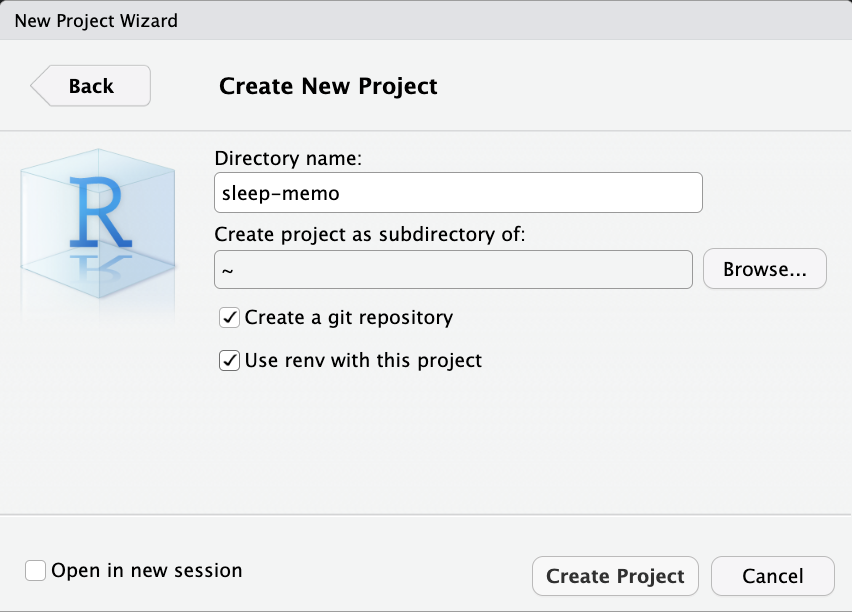
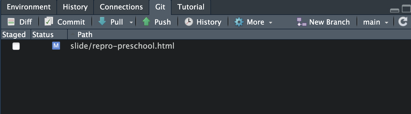
GitHub + RStudio Integration

You don’t have to use the terminal, RStudio has a built-in Git panel, you can:

• Clone a repo: File → New Project → Version Control

• Stage, commit, push, pull, browse history: use the Git tab

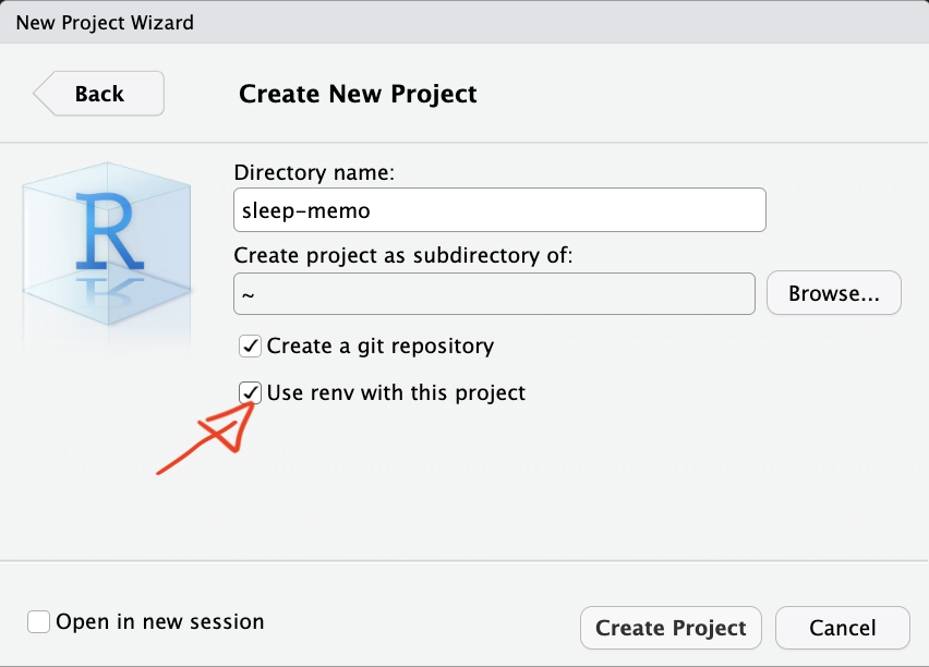
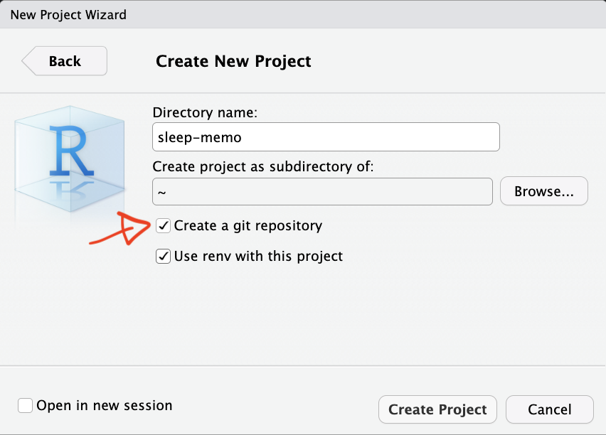
• New project with Git: tick “Create a git repository” at setup

Practice & resources

• Happy Git and GitHub for the useR
• GitHub Education: https://education.github.com
• Try GitHub Desktop (GUI client)

Start small. Use Git for one script. Then grow your skills from there.

I won’t lie: Git can be confusing at first. The terminology (commits, branches, merges, remotes) can feel overwhelming. But you don’t have to learn everything at once. Start simple: Use RStudio’s Git pane to commit and push; Learn how to clone, pull, and push Then explore branches and pull requests

If Git and GitHub feel too technical, or if your collaborators are less technical, the OSF is a fantastic alternative or complement.

• Upload data, code, and documents
• Create public or private projects
• Add collaborators
• Create preregistrations
• Generate DOIs for citation
• Track changes

You can also connect OSF to GitHub.

Integrated workflow 🛠️

1. Develop your analysis using R and Quarto.
   
2. Track code and scripts using Git.
   
3. Host your code on GitHub (public or private).
   
4. Upload your data and materials to OSF, including a data dictionary.
   
5. Link your GitHub repository to your OSF project.
   
6. Use renv for reproducible R environments.
   
7. Share the OSF project and cite it in your paper.

With this setup, anyone can: 1. Clone your repo 2. Restore your environment 3. Re-render your paper

Reproducibility

It’s about credibility and transparency.

Reproducible science is not about being perfect.

It’s about showing your work so that others can follow, understand, and build upon it.

Start simple, don’t wait until you’re “ready”, and teach what you learn!

You don’t need to become an expert overnight. You don’t have to adopt every tool I mentioned today all at once. Start small: Write your next data cleaning script with comments. Save your next analysis as an R Project. Try Quarto for your next report. Upload one dataset to OSF with a README. These little changes compound over time. And each time you do it, it gets easier. You’re not just changing your workflow. You’re investing in your future self.

THANK YOU!

References

Marwick, Ben, Carl Boettiger, and Lincoln Mullen. 2018. “Packaging Data Analytical Work Reproducibly Using r (and Friends).” The American Statistician 72 (1): 80–88. https://doi.org/10.1080/00031305.2017.1375986.

Reproducibility, Committee on, Replicability in Science, Board on Behavioral, Cognitive, and Sensory Sciences, Committee on National Statistics, Division of Behavioral, Social Sciences, Education, et al. 2019. Reproducibility and Replicability in Science. Washington, D.C.: National Academies Press. https://doi.org/10.17226/25303.

Wilkinson, Mark D., Michel Dumontier, IJsbrand Jan Aalbersberg, Gabrielle Appleton, Myles Axton, Arie Baak, Niklas Blomberg, et al. 2016. “The FAIR Guiding Principles for Scientific Data Management and Stewardship.” Scientific Data 3 (1): 160018. https://doi.org/10.1038/sdata.2016.18.