Introduction to Meta-Analysis with Application in R
PhD program in Psychological Sciences, University of Padova
2026-04-15
Course overview
- What is a meta-analysis?
- Effect sizes and their precision
- Meta-analytic models
- Heterogeneity
- Meta-regression
- Publication Bias
- Practice in R with
metafor
What is a meta-analysis?
Definition
Glass (1976) described meta-analysis as an “analysis of analyses”.
The aim of meta-analysis is to combine, summarize and interpret all available evidence pertaining to a clearly defined research question (Lipsey and Wilson 2001).
Systematic Reviews & Meta-Analysis
- A systematic review uses systematic and explicit methods to identify, select, and critically appraise relevant research.
- Meta-analysis refers to the use of statistical techniques to synthesize results across multiple primary studies (Hunt 1997).
A systematic review can be conducted without a statistical synthesis. A meta-analysis can be applied to data not retrieved via a systematic review (Crocetti 2016).
Systematic Review ↔︎ Meta-Analysis

Typical steps
Identify the research question. Is treatment X effective? Does effect Y exist?
Define inclusion/exclusion criteria. For example: randomized controlled trials, healthy participants, specific outcomes.
Systematically search for studies. Search the literature to identify all relevant studies.
Extract relevant information. Organize variables such as sample size, treatment type, age, and outcomes.
Summarize the results (systematic review). Provide a narrative summary with flowcharts, tables, and study characteristics.
Typical steps (continued)
Choose an effect size. Select a common metric to standardize results across studies.
Choose and fit a meta-analysis model. Implement the statistical model appropriate for the data.
Interpret and report the results.
The quality of the meta-analysis is the quality of included studies!
Why Meta-Analysis? (I)
The meta-analysis is a statistical procedure to combine multiple studies into a single statistical analysis (Borenstein et al. 2009; Hedges 2016):
- Switches the statistical unit from the single participant or observation (Level 1) to the study (Level 2)
- Combines evidence, assigning more weight to studies with lower estimation variability
- Using meta-regression, includes moderators to explain observed heterogeneity
This logic is analogous to how primary studies reason about individuals, only the scale changes.
Why Meta-Analysis? (II)
In a primary study, we sample subjects from a population and use the sample to make an inference to the population.
In meta-analysis, we sample studies from a universe of potential studies and use the sample to make an inference to that universe.
Credit: Filippo Gambarota
Effect sizes and their precision
How do we put studies on the same scale, and how certain are those estimates?
What we need for a Meta-Analysis
- An observed effect size (or outcome measure)
- Its precision (e.g., inverse of sampling variance)
The sampling variance depends on the effect size type and the study design (Veroniki et al. 2016; Borenstein et al. 2009), and is primarily driven by sample size. It is also common practice to apply a bias correction using Hedges’s \(g\) (Hedges 1981).
E.g., metafor::escalc(measure = "SMD") automatically applies the bias correction to standardized mean differences, returning Hedges’ g directly.
What is an effect size?
An effect size is a metric quantifying the direction and magnitude of the relationship between two entities.
- \(\theta_i\): the true effect size (unknown)
- \(\hat{\theta_i}\): the observed effect size for study \(i\), an estimate of \(\theta_i\)
\[\hat{\theta_i} = \theta_i + \epsilon_i\]
The observed effect deviates from the true effect because of sampling error \(\epsilon_i\) (the sampling variance is a measure of the sampling error).
An important part of estimation is estimating the magnitude of the sampling error in the estimate.
True vs. observed effect size
In every primary study, researchers can only draw a small sample from the whole population. Because a study can only sample from an infinitely large population, the observed effect will differ from the true population effect.
It is obviously desirable that \(\hat{\theta_i}\) is as close as possible to \(\theta_i\). Studies with smaller \(\epsilon_i\) deliver a more precise estimate and receive higher weight in meta-analysis.
Quantifying sampling error
The true effect \(\theta_i\) is unknown, and so \(\epsilon_i\) is also unknown. However, we can approximate the sampling error.
A common way to quantify \(\epsilon_i\) is through the standard error (SE), defined as the standard deviation of the sampling distribution.
i.e., the distribution of a statistic obtained by drawing random samples with the same \(n\) many times.
The sampling distribution
[1] 0.2836596
The SE of the mean
The standard error of the mean can be approximated by computing the ratio between the sample standard deviation to the square root of the sample size:
\[SE_{\bar{x}} = \frac{s}{\sqrt{n}}\]
This formula gives an approximation of the quantity we just estimated by simulation: the standard deviation of the sampling distribution of \(\bar{x}\) (mean).
SE shrinks with sample size
As \(n\) increases, the SE decreases and the study’s estimate of the true population mean becomes more precise (Harrer et al. 2021).
Code
n <- seq(2, 500, by = 1)

sammean <- function(n) {
  s  <- rnorm(n = n, mean = 10, sd = 2)
  m  <- mean(s)
  se <- sd(s) / sqrt(n)
  data.frame(n = n, m = m, se = se)
}

out <- lapply(n, sammean)
df  <- do.call(rbind, out)

me <- ggplot(df, aes(x = n, y = m)) +
  geom_ribbon(aes(ymin = m - se, ymax = m + se), alpha = 0.2) +
  geom_line() +
  geom_hline(yintercept = 10, linetype = "dashed", color = "red") +
  labs(x = "Sample size (n)", y = "Mean ± SE") +
  theme_clean(20)

se <- ggplot(df, aes(x = n, y = se)) +
  geom_line() +
  labs(x = "Sample size (n)", y = "SE") +
  theme_clean(20)

me | se
Effect sizes
In a primary study, it is easy to calculate effects because the outcome variable has been measured in the same way across all study subjects.
For example, studies using reaction times can calculate the difference between two conditions as \(\bar{X}_1 - \bar{X}_2\).
Another study addressing the same research question might use accuracy instead. We can still compute the difference between group means.
When two studies address the same question but use different outcome variables, their raw effects cannot be directly compared.
To perform a meta-analysis, we need an effect size that can be summarized across all studies.
Standardized effect sizes
The solution is to express all outcomes on a common metric that is interpretable regardless of the original scale. Meta-analysts often rely on standardized effect sizes, such as Cohen’s \(d\):
\[d = \frac{\bar{X}_1 - \bar{X}_2}{s_p}\]
\[s_p = \sqrt{\frac{(n_1-1)s_1^2 + (n_2-1)s_2^2}{n_1+n_2-2}}\]
Standardized effect sizes
A key distinction is whether the sampling variance of the estimator depends on the effect size itself (that can be an issue). For unstandardized effects this dependency is typically absent.
Unstandardized
\[V_d = \frac{s_1^2}{n_1} + \frac{s_2^2}{n_2}\]
Standardized
\[V_d = \frac{n_1 + n_2}{n_1\, n_2} + \frac{d^2}{2(n_1 + n_2)}\]
Each effect size has a specific formula for its sampling variability. The sample size is usually the most important information: studies with larger \(n\) have lower sampling variability.
Outcome measures
We can distinguish between measures used to:
- Contrast two independent groups (experimentally created or naturally occurring)
- Describe the direction and strength of association between two variables
- Summarize some characteristic or attribute of individual groups
- Quantify change within a single group or the difference between matched/paired samples
What outcome measure have we been using so far?
Adapted from escalc() documentation
(2) Pearson correlation
A correlation expresses the amount of linear co-variation between two continuous variables:
\[r_{xy} = \frac{\sigma_{xy}}{\sigma_x \, \sigma_y} \qquad SE_{r_{xy}} = \frac{1 - r^2_{xy}}{\sqrt{n-2}}\]
n <- 30 # n subj
r <- 0.7 # correlation
D <- diag(c(1, 1.2)) # standard deviation
R <- r + diag(1 - r, 2) # enter sd
S <- D %*% R %*% D # variance covarice matrix

# here we are doing the same as before for smd
cor_xy <- replicate(1e4, {
  xy <- MASS::mvrnorm(n = n, mu = c(0, .5), Sigma = S)
  cor(xy[, 1], xy[, 2])
  #sampling distribution of the correlation
})
Fisher’s z
Because most meta-analytic models assume normality, effect sizes are typically transformed before pooling. Correlations, which are bounded between −1 and 1, are therefore converted using Fisher’s z, which normalizes their sampling distribution and stabilizes their variance:
\[z = \frac{1}{2}\log\!\left(\frac{1+r}{1-r}\right) \qquad SE_z = \frac{1}{\sqrt{n-3}}\]
r vs. Fisher’s z
(4) Measures for change / matched pairs
Used when the goal is to quantify within-group change (e.g., pre–post treatment) or outcomes in matched/paired designs (Morris 2008; Borenstein et al. 2009).
- Standardized mean change, using pre-test SD, or pooled SD
- The pre–post correlation \(r_{pre,post}\) is needed to compute the correct sampling variance.
- Conduct a sensitivity analysis.
One simulated study
Steps:
- Generate two random samples from two normal distributions with a fixed mean difference
- Calculate the mean difference
- Repeat the same process many times
More specifically, we simulate an hypothetical study where two independent groups are compared:
\[\Delta = \overline{Y}_1 - \overline{Y}_2 \tag{1}\]
\[SE_\Delta = \sqrt{\frac{s_1^2}{n_1} + \frac{s_2^2}{n_2}} \tag{2}\]
With \(Y_{1_i} \sim \mathcal{N}(0,\, 1)\) and \(Y_{2_i} \sim \mathcal{N}(\Delta,\, 1)\).
In R
We assume both groups come from a normal distribution where \(g_1 \sim \mathcal{N}(0, 1)\) and \(g_2 \sim \mathcal{N}(D, 1)\). Using Equation 1 and Equation 2 we estimate the effect size and its variance.
The sim_umd() function wraps these steps for easy reuse:
Replicate 10,000 times
# return a list, n = 80, delta = 0.3
res <- replicate(1e4, sim_umd(n1 = 80, D = 0.3), simplify = FALSE)

# transform to dataframe
df  <- do.call(rbind, res)

nrow(df)
[1] 10000 yi vi
1 0.21288378 0.02603394
2 0.46087038 0.02556540
3 0.52595040 0.02497671
4 0.09124034 0.02298512
5 0.17137020 0.02335166
6 0.39134883 0.02850330The sampling distributions
Code
par(mfrow = c(1, 2))

hist(df$yi, breaks =20,
     main = expression("Sampling Distribution D"),
     xlab = "yi", col = my_cols[1], border = "white")
abline(v = mean(df$yi), lwd = 3)

hist(df$vi,breaks =20,
     main = expression("Sampling Distribution V"[D]),
     xlab = "vi", col = my_cols[2], border = "white")
abline(v = mean(df$vi), lwd = 3)
Which model would you choose if you were conducting a meta-analysis on this data?
Pooling effect sizes
Meta-analytic models differ in what they assume about the true effect size across studies.
What is the process through which these observed data were generated?
Meta-Analytic models
Equal-Effect Model
Assumes all studies share one single true effect \(\theta\). All observed variation is due only to sampling error.
Fixed-effect vs. equal-effect
Fixed-effect models allow each study to have its own fixed \(\theta_i\) (not necessarily equal across studies). The weighted average \(\bar{\theta}_w\) then summarises only the specific \(i\) studies included, inference is conditional and does not generalise to a broader population. The equal-effect model is the special case where \(\theta_i = \theta\) for all \(i\), which is the assumption that justifies population inference. The distinction is inferential, not computational.
Random-Effects Model
Assumes each study has its own true effect \(\theta_i\), sampled from a distribution around a grand mean \(\mu_\theta\).
Simulation setup
We start by generating simulated data from \(k\) studies.
For each simulated study (\(i\)),
we draw observations for two groups from normal distributions,
with the first group as \(g_{1i} \sim \mathcal{N}(0, 1)\) and
the second as \(g_{2i} \sim \mathcal{N}(D, 1)\).
From these, we calculate the estimated effect size (raw difference) and its sampling variance.
General function in R
sim_studies <- function(k, es, n1, n2 = NULL){
  if(length(n1) == 1) n1 <- rep(n1, k)
  if(is.null(n2)) n2 <- n1
  if(length(es) == 1) es <- rep(es, k)

  yi <- rep(NA, k)
  vi <- rep(NA, k)

  for(i in 1:k){
    g1 <- rnorm(n1[i], 0, 1)
    g2 <- rnorm(n2[i], es[i], 1)
    yi[i] <- mean(g2) - mean(g1)
    vi[i] <- var(g1)/n1[i] + var(g2)/n2[i]
  }

  sim <- data.frame(id = 1:k, yi, vi, n1 = n1, n2 = n2)

  # convert to escalc for using metafor method
  sim <- metafor::escalc(yi = yi, vi = vi, data = sim)

  return(sim)
}
Combining studies
Let’s imagine to have \(k = 10\) studies, a \(D = 0.5\) and heterogeneous sample sizes in each study.
   id     yi     vi n1 n2
1   1 0.2461 0.0621 23 23
2   2 0.5996 0.0701 29 29
3   3 0.4566 0.0634 32 32
4   4 0.3385 0.0920 25 25
5   5 0.6356 0.0687 34 34
6   6 0.0146 0.0968 25 25
7   7 1.0265 0.0451 29 29
8   8 0.4196 0.0432 40 40
9   9 0.4813 0.0573 32 32
10 10 0.7070 0.0716 33 33
The Equal-Effect (EE) Model
The equal-effect model assumes all studies share a single true effect \(\theta\) (i.e. D = 0.5), and the only source of variance is the within-study variance (i.e., \(v_i\)).
EE assumption
The assumptions are very simple:
there is a unique, true effect size to estimate \(\theta\),
each study is a more or less precise estimate of \(\theta\),
there is no TRUE variability among studies. The observed variability is due to studies that are imprecise (i.e., sampling error)
Based on previous assumptions and thinking a little bit, what could be the result of simulating studies with a very large \(n\)?
EE model formally
Assume \(i = 1, \ldots, k\) independent studies, where \(y_i\) is the observed effect size and \(\theta\) the single shared true effect, such that:
\[y_i = \theta + \epsilon_i, \quad \epsilon_i \sim \mathcal{N}(0, \sigma^2_i)\]
All studies estimate the same \(\theta\). The sampling variances \(\sigma^2_i\) are assumed known (estimated analytically from each study’s data, \(v_i\)).
Weighting studies
We want to consider that some studies, despite providing a similar effect size could give more information. An higher sample size (or lower sampling variance) produce a more reliable estimation.
Would you trust more a study with \(n = 100\) and \(D = 0.5\) or a study with \(n = 10\) and \(D = 0.5\)?
EE model as a weighted average
With weighted estimation (method = "EE" in metafor), the model estimates \(\theta\) via an inverse-variance weighted average:
\[\hat{\theta}_w = \frac{\sum_{i=1}^{k} w_i y_i}{\sum_{i=1}^{k} w_i}, \quad w_i = \frac{1}{v_i}\]
\[SE_{\hat{\theta}_w} = \sqrt{\frac{1}{\sum_{i=1}^{k} w_i}}\]
Fitting an EE model
The model can be fitted using the metafor::rma() function, with method = "EE".
Equal-Effects Model (k = 10)

  logLik  deviance       AIC       BIC      AICc
 -1.0150   10.9816    4.0299    4.3325    4.5299

I^2 (total heterogeneity / total variability):   18.04%
H^2 (total variability / sampling variability):  1.22

Test for Heterogeneity:
Q(df = 9) = 10.9816, p-val = 0.2770

Model Results:

estimate      se    zval    pval   ci.lb   ci.ub
  0.5266  0.0794  6.6325  <.0001  0.3710  0.6823  ***

---
Signif. codes:  0 '***' 0.001 '**' 0.01 '*' 0.05 '.' 0.1 ' ' 1
Interpreting an EE model
- The first section (
logLik,deviance, etc.) presents general model statistics and information criteria - The \(I^2\) and \(H^2\) evaluate the observed heterogeneity (see next slides)
- The
Test of Heterogeneitypresents the \(Q\) statistic (a significant result suggests the equal-effect assumption may be violated) - The
Model Resultssection presents \(\hat{\theta}_w\) with standard error and the Wald \(z\) test (\(H_0 : \theta = 0\))
The metafor package has several well documented functions to calculate and plot model results, residuals analysis etc.
Interpreting an EE model
Are the EE sssumptions realistic?
If we relax the assumption that all \(\theta_i\) are equal, we are able to combine studies that are not exact replications.
Thus the true effect is no longer a single value shared across studies, but can be larger or smaller depending on conditions.
In other terms we are assuming that there could be some variability (i.e., heterogeneity) among studies that is independent from the sample size. Even with studies with \(\lim_{n \to \infty}\) the observed variability is not zero.
The Random-Effects Model (RE)
The random-effects model assumes that the true effects are normally distributed across studies.
“The goal of the random-effects model is therefore not to estimate the one true effect size of all studies, but the mean of the distribution of true effects.” (Harrer et al. 2021)
We need to estimate:
- \(\mu_\theta\): mean of the distribution = average effect size across different true effect sizes
- \(\tau^2\): variance of the distribution = variability / heterogeneity of effect sizes
In practical terms, we now have two sources of variability: \(\tau^2\) (real differences among effect sizes) and \(\sigma^2_i\) (known sampling variance of each study).
If we were dealing with means, what would our \(\sigma^2_i\) be?
We can extend the fixed-effect model including \(\tau^2\). \(\tau^2\) is the true heterogeneity among studies caused by methodological differences or intrinsic variability in the phenomenon.
Formally we can extend FE model as:
\[y_i = \mu_\theta + \delta_i + \epsilon_i\]
\[\delta_i \sim \mathcal{N}(0, \tau^2)\]
\[\epsilon_i \sim \mathcal{N}(0, \sigma^2_i)\]
Where \(\mu_\theta\) is the average effect size and \(\delta_i\) is the study-specific deviation from the average effect (regulated by \(\tau^2\)). Each study specific effect is \(\theta_i = \mu_\theta + \delta_i\).
Exchangeability
- All true effect sizes \(\theta_i = \mu_\theta + \delta_i\) are considered exchangeable: before observing the data, we have no basis for predicting study-specific deviations (Higgins, Thompson, and Spiegelhalter 2009).
- The magnitude of \(\delta_i\) is independent of the study. Nothing tells us a priori whether \(\delta_i\) will be large or small in any given study.
- If study design or context systematically predicts the direction of \(\delta_i\), exchangeability is violated and meta-regression it’s probably needed.
RE model estimation
The RE model is still a weighted average, but weights now include \(\tau^2\) to account for between-study heterogeneity:
\[\hat{\theta}_w = \frac{\sum_{i=1}^{k} y_i w_i^*}{\sum_{i=1}^{k} w_i^*}\]
\[w_i^* = \frac{1}{\sigma^2_i + \tau^2}\]
Large studies
\(\sigma^2_i \approx 0\), so adding \(\tau^2\) substantially increases total variance: weight is pulled down relative to FE
Small studies
\(\sigma^2_i\) is large, so \(\tau^2\) adds proportionally less: weight is pulled up relative to FE
As the number of studies \(k\) increases, the estimation of \(\mu_\theta\) and \(\tau^2\) becomes more precise (Borenstein et al. 2009).
As the sample size of each study increases, each \(\mu_\theta + \delta_i\) is estimated with higher precision. However, as long as \(\tau^2 \neq 0\), there will still be variability among effect sizes.
Increasing the sample size of each study or the number of studies does not affect the value of \(\tau^2\), only its estimation precision (Gambarota and Altoè 2024)
Simulating a RE model
To simulate the RE model we simply need to include \(\tau^2\) in the equal-effect model simulation.
k <- 20 # number of studies
mu <- 0.5 # average effect
tau2 <- 0.1 # heterogeneity
n <- 10 + rpois(k, 30 - 10) # sample size
deltai <- rnorm(k, 0, sqrt(tau2)) # random-effects
thetai <- mu + deltai # true study effect
# now we have an effect for each study, we are not assuming equality
dat <- sim_studies(k = k, es = thetai, n1 = n)
head(dat)
  id     yi     vi n1 n2
1  1 0.2603 0.0699 31 31
2  2 0.3974 0.0565 34 34
3  3 0.3738 0.0608 33 33
4  4 0.0937 0.0476 33 33
5  5 0.4933 0.0608 39 39
6  6 0.6814 0.0546 33 33
Insert everything into a function:
sim_studies <- function(k, es, tau2 = 0, n1, n2 = NULL, add = NULL){
  if(length(n1) == 1) n1 <- rep(n1, k)
  if(is.null(n2)) n2 <- n1
  if(length(es) == 1) es <- rep(es, k)

  yi <- rep(NA, k)
  vi <- rep(NA, k)

  # random effects
  deltai <- rnorm(k, 0, sqrt(tau2))

  for(i in 1:k){
    g1 <- rnorm(n1[i], 0, 1)
    g2 <- rnorm(n2[i], es[i] + deltai[i], 1)
    yi[i] <- mean(g2) - mean(g1)
    vi[i] <- var(g1)/n1[i] + var(g2)/n2[i]
  }

  sim <- data.frame(id = 1:k, yi, vi, n1 = n1, n2 = n2)

  if(!is.null(add)){ # we will need this later
    sim <- cbind(sim, add)
  }

  # convert to escalc for using metafor
  sim <- metafor::escalc(yi = yi, vi = vi, data = sim)

  return(sim)
}
Fitting a RE model
In R we can use the metafor::rma() function using the method = "REML".
Random-Effects Model (k = 20; tau^2 estimator: REML)
logLik deviance AIC BIC AICc
-5.7558 11.5116 15.5116 17.4005 16.2616
tau^2 (estimated amount of total heterogeneity): 0.0410 (SE = 0.0326)
tau (square root of estimated tau^2 value): 0.2026
I^2 (total heterogeneity / total variability): 41.01%
H^2 (total variability / sampling variability): 1.70
Test for Heterogeneity:
Q(df = 19) = 32.6253, p-val = 0.0265
Model Results:
estimate se zval pval ci.lb ci.ub
0.4079 0.0713 5.7212 <.0001 0.2682 0.5477 ***
---
Signif. codes: 0 '***' 0.001 '**' 0.01 '*' 0.05 '.' 0.1 ' ' 1
To see the actual impact of \(\tau^2\) we can follow the same approach using a large \(n\). The sampling variance vi of each study is basically 0.
# ... other parameters as before
n <- 1e4
dat <- sim_studies(k = k, es = mu, tau2 = tau2, n1 = n)
head(dat)
id yi vi n1 n2
1 1 0.8803 0.0002 10000 10000
2 2 0.4661 0.0002 10000 10000
3 3 0.7462 0.0002 10000 10000
4 4 0.8856 0.0002 10000 10000
5 5 -0.0218 0.0002 10000 10000
6 6 0.2230 0.0002 10000 10000 Fitting a RE model
In R we can use the metafor::rma() function using the method = "REML".
Random-Effects Model (k = 20; tau^2 estimator: REML)
logLik deviance AIC BIC AICc
-2.8353 5.6705 9.6705 11.5594 10.4205
tau^2 (estimated amount of total heterogeneity): 0.0787 (SE = 0.0256)
tau (square root of estimated tau^2 value): 0.2806
I^2 (total heterogeneity / total variability): 99.75%
H^2 (total variability / sampling variability): 396.50
Test for Heterogeneity:
Q(df = 19) = 7540.8016, p-val < .0001
Model Results:
estimate se zval pval ci.lb ci.ub
0.4450 0.0628 7.0839 <.0001 0.3219 0.5681 ***
---
Signif. codes: 0 '***' 0.001 '**' 0.01 '*' 0.05 '.' 0.1 ' ' 1
Other complex (but common) models
Heterogeneity
Assessing heterogeneity
This requires addressing two questions:
Is there significant heterogeneity across studies?
How large is this heterogeneity?
Borenstein (2024)
Observed vs. true effects
As we said, in a meta-analysis, we distinguish between two versions of the effect size:
- True effect size \(\theta_i\): the effect we would see if we could remove sampling error (e.g., enroll the entire population)
- Observed effect size \(\hat{\theta}_i\): what is actually observed in the sample, inevitably over- or underestimates \(\theta_i\)
The distribution of observed effects tends to be wider than the distribution of true effects.
To understand why, consider a hypothetical example where all studies are random samples from the same population and identical in all material respects. Since all studies estimate the same true effect, \(\tau^2 = 0\) by definition. Yet the observed effects still vary because of sampling error.
\[V_{OBS} = \tau^2 + V_{ERR}\]
The Q Test
If we could remove the sampling error, would the effect size be identical in all studies?
The Q-test only tells us whether heterogeneity exists, not how much.
Can be considered as a weighted sum of squares:
\[Q = \sum_{i=1}^{k} w_i \left(y_i - \hat{\mu}\right)^2\] With, \(y_i\) is the observed effect of study \(i\), \(\hat{\mu}\) is the pooled effect.
Each study’s residual \((y_i - \hat{\mu})\) is weighted by precision \(w_i\) and summed across all \(k\) studies.
The value of \(Q\) depends on both the magnitude of deviations and the precision of studies.
A study with high precision gives a larger weight to even small deviations from \(\hat{\mu}\), inflating \(Q\).
The \(Q\) statistics
Check if there is excess variation in our data, meaning more variation than can be expected from sampling error alone.
Being a sum of squared distances, \(Q\) follows approximately a \(\chi^2\) distribution with \(df = k - 1\).
No heterogeneity (\(\tau^2 = 0\))
Variability is due to sampling error only. The expected value of \(Q\) equals the degrees of freedom:
\[\mathbb{E}[Q] = k - 1\]
True heterogeneity (\(\tau^2 \neq 0\))
\(Q\) follows a non-central \(\chi^2\) with non-centrality parameter \(\lambda\):
\[\mathbb{E}[Q] = k - 1 + \lambda\]
If the observed \(Q\) exceeds what we would expect under no heterogeneity (\(df = K-1\)), we have evidence that \(\tau^2 \neq 0\) — i.e., that true between-study heterogeneity exists.
Code
set.seed(42)
N_sim <- 2000
K <- 30
sigma_k <- runif(K, 0.1, 0.4) # per-study SEs
w_k <- 1 / sigma_k^2 # inverse-variance weights
simulate_meta <- function(tau2) {
Q_vals <- numeric(N_sim)
res_vals <- numeric(N_sim * K)
for (i in seq_len(N_sim)) {
u_k <- rnorm(K, 0, sqrt(tau2))
theta_k <- rnorm(K, u_k, sigma_k)
theta_hat <- sum(w_k * theta_k) / sum(w_k)
Q_vals[i] <- sum(w_k * (theta_k - theta_hat)^2)
res_vals[seq((i - 1) * K + 1, i * K)] <- theta_k - theta_hat
}
list(Q = Q_vals, res = res_vals)
}
sim0 <- simulate_meta(0)
sim01 <- simulate_meta(0.1)
plot_Q <- function(Q_vals, tau2_label) {
x_seq <- seq(0, 150, length.out = 500)
chi2_df <- data.frame(x = x_seq, y = dchisq(x_seq, df = K - 1))
ggplot(data.frame(Q = Q_vals), aes(Q)) +
geom_histogram(aes(y = after_stat(density)),
bins = 40, fill = "grey75", colour = "white") +
geom_line(data = chi2_df, aes(x, y),
colour = my_cols[2], linewidth = 2) +
scale_x_continuous(limits = c(0, 150)) +
labs(title = bquote(tau^2 == .(tau2_label)), x = "Q", y = "Density") +
theme_clean(18)
}
sd_r <- sd(sim0$res)
plot_res <- function(res_vals, tau2_label) {
x_seq <- seq(-2, 2, length.out = 500)
norm_df <- data.frame(x = x_seq, y = dnorm(x_seq, 0, sd_r))
ggplot(data.frame(r = res_vals), aes(r)) +
geom_histogram(aes(y = after_stat(density)),
bins = 50, fill = "grey75", colour = "white") +
geom_line(data = norm_df, aes(x, y),
colour = my_cols[3], linewidth = 2) +
labs(title = bquote(tau^2 == .(tau2_label)),
x = expression(y[i] - hat(mu)), y = "Density") +
theme_clean(18)
}
(plot_Q(sim0$Q, 0) | plot_res(sim0$res, 0)) /
(plot_Q(sim01$Q, 0.1) | plot_res(sim01$res, 0.1))
Warnings
If there are few studies in the meta-analysis, the \(Q\)−test is likely underpowered for detecting true heterogeneity
Conversely, \(Q\)-test has too much power if the number of studies is large
\(Q\)-test should be evaluated together with forest plot and other indices of heterogeneity
The \(I^2\) statistic (Higgins and Thompson 2002)
Of the variance we see, what proportion reflects variance in true effects rather than sampling variance?
\[I^2 = \frac{\tau^2}{\tau^2 + \sigma^2}\]
It’s not an absolute measure of heterogeneity, it’s the ratio of true to total observed variance.
\(I^2\) quantifies how much of the total variability in effect sizes is not caused by sampling error, expressed as a percentage.
It builds directly on \(Q\), exploiting the fact that \(\mathbb{E}[Q] = k-1\) under \(\tau^2 = 0\):
\[I^2 = \frac{Q - (k-1)}{Q}\]
- Numerator \(Q-(k-1)\): excess variation beyond what sampling error alone predicts
- Denominator \(Q\): total observed variation
\(I^2\) in metafor
\(I^2\) is derived from the estimated between-study variance \(\hat{\tau}^2\):
\[I^2 = \frac{\hat{\tau}^2}{\hat{\tau}^2 + \tilde{v}}\]
where \(\tilde{v}\) is the “typical” sampling variance (\(\sigma^2\)) across all \(k\) studies:
\[\tilde{v} = \frac{(k-1)\displaystyle\sum w_i}{\left(\displaystyle\sum w_i\right)^2 - \displaystyle\sum w_i^2}\] where \(w_i = 1/v_i\) is the inverse of the sampling variance of the \(i^{th}\) study.
\(I^2\) depends on \(\tilde{v}\), which varies from meta-analysis to meta-analysis. Two meta-analyses with the same \(\tau^2\) but different study precisions can yield very different \(I^2\) values (Borenstein 2022)!
Large studies (small \(\tilde{v}\)): Even a irrelevant \(\tau^2\) can produce a large \(I^2\), because sampling variance is tiny relative to true-effect variance.
Small studies (large \(\tilde{v}\)): \(I^2\) may stay small even when true-effect differences are large, because sampling variance dominates the denominator.
The \(H^2\) statistic
\(H^2\) is an alternative index of heterogeneity:
\[H^2 = \frac{Q}{k - 1}\]
- \(Q\): weighted sum of squares: total observed variability
- \(k-1\): expected value of \(Q\) under \(\tau^2 = 0\)
So \(H^2\) is the ratio of total heterogeneity to the sampling variability expected under the null.
Interpretation
| \(H^2\) | Meaning |
|---|---|
| \(= 1\) | No excess heterogeneity (\(Q = k-1\)) |
| \(> 1\) | More variability than expected from sampling error alone |
Higher \(H^2\) \(\Rightarrow\) higher heterogeneity relative to sampling variability.
Like \(I^2\), \(H^2\) is not a measure of absolute heterogeneity.
k <- 10 # number of studies
mu <- 0.5 # average effect
tau2 <- 0.1 # heterogeneity
n <- 10 + rpois(k, 30 - 10) # sample size
dat <- sim_studies(k = k, es = mu, tau2 = tau2, n1 = n) #simulate data
fit <- rma(yi, vi, data = dat, method = "REML")
summary(fit)
Random-Effects Model (k = 10; tau^2 estimator: REML)
logLik deviance AIC BIC AICc
-5.1308 10.2616 14.2616 14.6561 16.2616
tau^2 (estimated amount of total heterogeneity): 0.1062 (SE = 0.0837)
tau (square root of estimated tau^2 value): 0.3259
I^2 (total heterogeneity / total variability): 60.23%
H^2 (total variability / sampling variability): 2.51
Test for Heterogeneity:
Q(df = 9) = 22.4669, p-val = 0.0075
Model Results:
estimate se zval pval ci.lb ci.ub
0.5063 0.1334 3.7968 0.0001 0.2449 0.7677 ***
---
Signif. codes: 0 '***' 0.001 '**' 0.01 '*' 0.05 '.' 0.1 ' ' 1k <- 10 # number of studies
mu <- 0.5 # average effect
tau2 <- 0.01 # heterogeneity
n <- rep(1e4, k) # sample size
dat <- sim_studies(k = k, es = mu, tau2 = tau2, n1 = n) #simulate data
fit <- rma(yi, vi, data = dat, method = "REML")
summary(fit)
Random-Effects Model (k = 10; tau^2 estimator: REML)

  logLik  deviance       AIC       BIC      AICc
  5.7988  -11.5976   -7.5976   -7.2031   -5.5976

tau^2 (estimated amount of total heterogeneity): 0.0159 (SE = 0.0076)
tau (square root of estimated tau^2 value):      0.1262
I^2 (total heterogeneity / total variability):   98.76%
H^2 (total variability / sampling variability):  80.75

Test for Heterogeneity:
Q(df = 9) = 724.8237, p-val < .0001

Model Results:

estimate      se     zval    pval   ci.lb   ci.ub
  0.4824  0.0402  12.0091  <.0001  0.4037  0.5612  ***

---
Signif. codes:  0 '***' 0.001 '**' 0.01 '*' 0.05 '.' 0.1 ' ' 1
Open questions:
- Over what interval is the effect size expected to fall?
- Is the effect always small, or are there studies where the effect is large?
- Is the effect always a decrease in mortality, or are there studies where the effect is an increase in mortality?
In other words, we are asking about heterogeneity in a clinical/practical context, not just a statistical one (Borenstein 2024).
Variance \(\tau^2\) and standard deviation \(\tau\)
Remeber the RE formula:
\[y_i = \mu_\theta + \delta_i + \epsilon_i\]
\[\delta_i \sim \mathcal{N}(0, \tau^2)\]
\[\epsilon_i \sim \mathcal{N}(0, \sigma^2_i)\]
Where \(\mu_\theta\) is the average effect size and \(\delta_i\) is the study-specific deviation from the average effect (regulated by \(\tau^2\)). So \(\tau^2\) is just the variance of the random-effect. This means that we can intepret it as the variability (or the standard deviation, \(\tau\)) of the true effect size distribution.
\(\tau\) is expressed on the same scale as the effect size metric, interpretable like a standard deviation in a primary study. The value of \(\tau\) tells us about the range of the true effect sizes.
Confidence intervals
What is reported in the model summary as ci.lb and ci.ub refers to the 95% confidence interval representing the uncertainty in estimating the effect.
Random-Effects Model (k = 10; tau^2 estimator: REML)

tau^2 (estimated amount of total heterogeneity): 0.0159 (SE = 0.0076)
tau (square root of estimated tau^2 value):      0.1262
I^2 (total heterogeneity / total variability):   98.76%
H^2 (total variability / sampling variability):  80.75

Test for Heterogeneity:
Q(df = 9) = 724.8237, p-val < .0001

Model Results:

estimate      se     zval    pval   ci.lb   ci.ub
  0.4824  0.0402  12.0091  <.0001  0.4037  0.5612  ***

---
Signif. codes:  0 '***' 0.001 '**' 0.01 '*' 0.05 '.' 0.1 ' ' 1
Is it \(\tau^2\) involved in the computation of confidence intervals?
Without looking at the equations, let’s try to obtain the results via simulations:
nsim <- 5e3
k <- 20 # number of studies
mu <- 0.5 # average effect
tau2 <- 0.05 # heterogeneity
n <- 50 # sample size

mui <- rep(NA, nsim)#init vector
for(i in 1:nsim){
  dat <- sim_studies(k = k, es = mu, tau2 = tau2, n1 = n) #simulate dat
  fit <- rma(yi, vi, data = dat)
  mui[i] <- coef(fit)[1] #extract estimate
}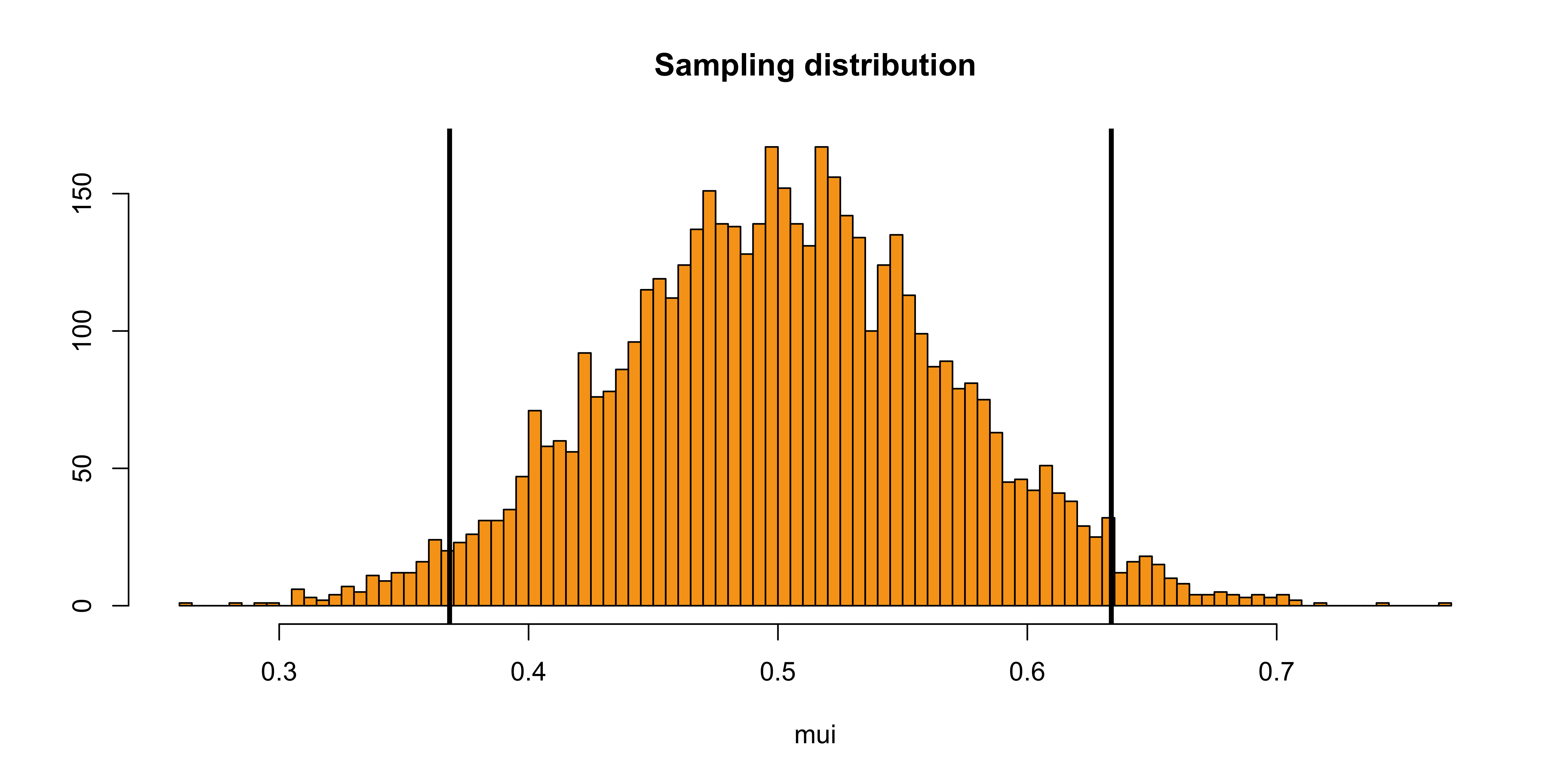
The 95% CI around the pooled effect uses a standard error that is a function of within-study sampling variances (driven mainly by \(n\)), \(\tau^2\), and \(k\):
\[CI = \hat{\mu}_\theta \pm z_\alpha \times SE_{\mu_\theta}\]
\[SE_{\mu_\theta} = \sqrt{\frac{1}{\displaystyle\sum_{i=1}^{k} w_i^\star}}\]
\[w_i^\star = \frac{1}{\sigma_i^2 + \tau^2}\]
What drives the CI width?
| Factor | Effect on \(SE\) |
|---|---|
| \(\uparrow k\) (more studies) | \(SE \downarrow\) |
| \(\uparrow \tau^2\) (more heterogeneity) | \(SE \uparrow\) |
| \(\uparrow n_i\) (larger studies, smaller \(\sigma_i^2\)) | \(SE \downarrow\) |
Confidence vs. prediction intervals
The CI speaks to the location of the mean effect in the universe of comparable studies. The PI speaks to the dispersion of those effects (IntHout et al. 2016; Borenstein 2024).
In meta-analysis, if we knew the true mean \(\mu_\theta\) and the SD of true effects \(\tau\), the 95% PI would simply be (Viechtbauer 2007):
\[PI = \mu_\theta \pm 1.96 \times \tau\]
If true effects vary across studies with standard deviation \(\tau\), then the true effect in a new similar study is expected to fall within about \(1.96 \times \tau\) units above or below the average true effect.
Where does \(PI = \mu_\theta \pm 1.96 \times \tau\) come from?
True effects vary across studies: \(\theta \sim N(\mu_\theta,\ \tau^2)\)
Standardize: subtract mean, divide by SD:
\[Z = \frac{\theta - \mu_\theta}{\tau} \sim N(0,1) \quad\Longrightarrow\quad \theta = \mu_\theta + Z \cdot \tau\]
Back-transform the 97.5th quantile of \(Z\), i.e. \(z_{0.975} = 1.96\):
\[\theta_{0.975} = \mu_\theta + \underbrace{1.96}_{\substack{\text{Z quantile}}} \times \underbrace{\tau}_{\substack{\text{rescales back}\\\text{to } \theta\text{ scale}}}\]
Given that we don’t know the true mean \(\mu_\theta\) and \(\tau\), to obtain the interval we have to use both between-study heterogeneity and the estimation error:
\[PI = \hat{\mu}_\theta \pm z_\alpha\sqrt{\hat{\tau}^2 + SE^2_{\mu_\theta}}\]
CI vs. PI
| CI | PI | |
|---|---|---|
| Uncertainty about | \(\hat{\mu}_\theta\) | A new true effect |
| Width when \(\tau^2 = 0\) | Same as PI | Same as CI |
| Width when \(\tau^2 > 0\) | Narrower | Wider |
Practical implication
The PI answers the pratical relevant question: “What effect size would we expect in the next study?” The CI only tells us how well we estimated the average effect.
Meta-regression
Meta-regression
To explain heterogeneity, study-level predictor variables can be specified
In this case, a mixed-effects model (i.e., Meta-Regression) will be performed
In
rma(), study-level predictors (categorical and/or quantitative) can be specified via themodargument
Until now, we have seen Equal-Effects and Random-Effects models as intercept-only linear regression.
The pooled effect is simply the intercept.
Equal-Effects (EE) model
\(\beta_0\) is \(\theta\) and \(\epsilon_i \sim \mathcal{N}(0, \sigma_i^2)\):
\[y_i = \beta_0 + \epsilon_i\]
Each study contributes a noisy observation of the single true effect \(\theta\).
Random-Effects (RE) model
\(\beta_0\) is \(\mu_\theta\) and the study-specific random intercepts \(\beta_{0_i}\) are the \(\delta_i\):
\[y_i = \beta_0 + \beta_{0_i} + \epsilon_i, \quad \beta_{0_i} \sim \mathcal{N}(0, \tau^2)\]
Studies are allowed to have their own true effect, distributed around the grand mean \(\mu_\theta\).
Explaining \(\tau^2\)
So far we have either assumed \(\tau^2 = 0\) (EE model) or estimated it without explanation (RE model).
We can extend the intercept-only meta-analysis by including study-level predictors (just as in standard linear regression) to explain the estimated true heterogeneity.
Example
\(k = 100\) studies, measuring the same effect, but:
- 50 studies are lab-based experiments (\(x_{lab}\))
- 50 studies are online experiments (\(x_{online}\))
We hypothesize that the type of experiment moderates the true effect size.
\[\tau^2 - \tau^2_r = \text{variance explained by } X\]
Adding \(X\) to the model should reduce \(\tau^2\) if \(X\) is a genuine moderator.
The Meta-Regression
With a predictor \(x\) (type of experiment) and treatment coding (type coded 0 = lab, 1 = online):
\[y_i = \beta_0 + \beta_{0_i} + \beta_1 X_i + \epsilon_i\]
with:
\[y_{\text{lab}_i} = \beta_0 + \beta_{0_i} + \epsilon_i\]
\[y_{\text{online}_i} = \beta_0 + \beta_{0_i} + \beta_1 + \epsilon_i\]
Parameter interpretation
| Parameter | Meaning |
|---|---|
| \(\beta_0\) | Effect size when \(X = 0\) (lab-based) |
| \(\beta_1\) | Difference: online \(-\) lab |
| \(\beta_0 + \beta_1\) | Effect size for online studies |
NB. The meaning of the parameters depends on the coding. With treatment coding, \(\beta_0\) is always the effect for the reference category (\(X = 0\)). Other codings (e.g., sum coding) yield different intercept interpretations.
Explaining \(\tau^2\)
Adding a predictor does not remove between-study variability entirely.
The random effect \(\beta_{0_i}\) (ie., \(\delta_i\)) is still present, but now captures only residual heterogeneity \(\tau^2_r\):
\[y_i = \beta_0 + \beta_{0_i} + \beta_1 X_i + \epsilon_i \tag{3}\]
\[\beta_{0_i} \sim \mathcal{N}(0,\ \tau^2_r)\]
Before vs. after adding \(X\)
- Without predictor: \(\beta_{0_i} \sim \mathcal{N}(0, \tau^2)\) — total heterogeneity
- With predictor: \(\beta_{0_i} \sim \mathcal{N}(0, \tau^2_r)\) — residual heterogeneity
Pseudo \(R^2\)
The proportion of heterogeneity explained by \(X\):
\[R^2 = 1- \frac{\tau^2_r}{\tau^2}\]
This is reported by metafor::rma() as pseudo \(R^2\).
Simulating the \(X\) effect
To simulate a meta-regression we choose \(\beta_0\) and \(\beta_1\) and implement Equation 3. With treatment coding, \(\beta_0\) is the lab effect size and \(\beta_1\) is the lab–online difference.
k <- 100
b0 <- 0.3   # lab-based effect size
b1 <- 0.5   # online - lab-based

type <- rep(c("lab", "online"), each = k/2)
type_dummy <- ifelse(type == "lab", 0, 1)   # treatment coding
es  <- b0 + b1 * type_dummy

data.frame(type = type, es = es)
type es
1 lab 0.3
2 lab 0.3
3 lab 0.3
4 lab 0.3
5 lab 0.3
6 lab 0.3
7 lab 0.3
8 lab 0.3
9 lab 0.3
10 lab 0.3
11 lab 0.3
12 lab 0.3
13 lab 0.3
14 lab 0.3
15 lab 0.3
16 lab 0.3
17 lab 0.3
18 lab 0.3
19 lab 0.3
20 lab 0.3
21 lab 0.3
22 lab 0.3
23 lab 0.3
24 lab 0.3
25 lab 0.3
26 lab 0.3
27 lab 0.3
28 lab 0.3
29 lab 0.3
30 lab 0.3
31 lab 0.3
32 lab 0.3
33 lab 0.3
34 lab 0.3
35 lab 0.3
36 lab 0.3
37 lab 0.3
38 lab 0.3
39 lab 0.3
40 lab 0.3
41 lab 0.3
42 lab 0.3
43 lab 0.3
44 lab 0.3
45 lab 0.3
46 lab 0.3
47 lab 0.3
48 lab 0.3
49 lab 0.3
50 lab 0.3
51 online 0.8
52 online 0.8
53 online 0.8
54 online 0.8
55 online 0.8
56 online 0.8
57 online 0.8
58 online 0.8
59 online 0.8
60 online 0.8
61 online 0.8
62 online 0.8
63 online 0.8
64 online 0.8
65 online 0.8
66 online 0.8
67 online 0.8
68 online 0.8
69 online 0.8
70 online 0.8
71 online 0.8
72 online 0.8
73 online 0.8
74 online 0.8
75 online 0.8
76 online 0.8
77 online 0.8
78 online 0.8
79 online 0.8
80 online 0.8
81 online 0.8
82 online 0.8
83 online 0.8
84 online 0.8
85 online 0.8
86 online 0.8
87 online 0.8
88 online 0.8
89 online 0.8
90 online 0.8
91 online 0.8
92 online 0.8
93 online 0.8
94 online 0.8
95 online 0.8
96 online 0.8
97 online 0.8
98 online 0.8
99 online 0.8
100 online 0.8Then simulate observed effects with sim_studies(), passing es as a vector and setting tau2 to the residual heterogeneity \(\tau^2_r\):
tau2r <- 0.05   # residual heterogeneity after accounting for X
n <- 10 + rpois(k, 30 - 10) # sample size

dat <- sim_studies(k = k, es = es, tau2 = tau2r, n1 = n,
                     add = list(type = type))
head(dat, n = 3); tail(dat, n = 3)
  id      yi     vi n1 n2 type
1  1 -0.1634 0.0746 23 23  lab
2  2  0.2757 0.0641 26 26  lab
3  3  0.0375 0.0623 38 38  lab
     id     yi     vi n1 n2   type
98   98 1.0197 0.0688 27 27 online
99   99 0.9334 0.0653 22 22 online
100 100 0.4222 0.0751 26 26 online
Fitting a meta-regression
Meta-regression uses metafor::rma() with the mods = ~ argument — the right-hand side of a y ~ x formula, exactly as in lm(). The predictor name must match a column in the data dataframe.
Mixed-Effects Model (k = 100; tau^2 estimator: REML)

tau^2 (estimated amount of residual heterogeneity):     0.0286 (SE = 0.0137)
tau (square root of estimated tau^2 value):             0.1691
I^2 (residual heterogeneity / unaccounted variability): 29.73%
H^2 (unaccounted variability / sampling variability):   1.42
R^2 (amount of heterogeneity accounted for):            65.28%

Test for Residual Heterogeneity:
QE(df = 98) = 139.4219, p-val = 0.0038

Test of Moderators (coefficient 2):
QM(df = 1) = 55.8691, p-val < .0001

Model Results:

            estimate      se    zval    pval   ci.lb   ci.ub
intrcpt       0.3202  0.0444  7.2099  <.0001  0.2332  0.4072  ***
typeonline    0.4670  0.0625  7.4746  <.0001  0.3446  0.5895  ***

---
Signif. codes:  0 '***' 0.001 '**' 0.01 '*' 0.05 '.' 0.1 ' ' 1
intrcpt and typeonline are the estimates of \(\beta_0\) and \(\beta_1\). Their interpretation depends on the effect size scale and the contrast coding used.
| Term | Estimate | Interpretation |
|---|---|---|
intrcpt |
0.3202 | Lab-based ES (\(X=0\)) |
typeonline |
0.4670 | Online \(-\) lab difference |
| Sum | 0.7872 | Online ES (\(X=1\)) |
True values: \(\beta_0 = 0.3\), \(\beta_1 = 0.5\)
Interpreting the output
The rma() output is similar to the RE model with a few key additions:
- All heterogeneity statistics (\(H^2\), \(I^2\), \(Q\), \(\tau^2\)) now refer to residual heterogeneity — the variability left unexplained after accounting for \(X\)
- A pseudo \(R^2\) quantifies the proportion of \(\tau^2\) explained by the moderator
- A \(Q_M\) omnibus test tests whether all moderator coefficients are jointly zero
- A coefficient table (similar to
lm()) reports \(\hat{\beta}\), SE, and Wald \(z\)-test for each parameter
Omnibus moderator test (\(Q_M\))
Mixed-Effects Model (k = 100; tau^2 estimator: REML)

tau^2 (estimated amount of residual heterogeneity):     0.0286 (SE = 0.0137)
tau (square root of estimated tau^2 value):             0.1691
I^2 (residual heterogeneity / unaccounted variability): 29.73%
H^2 (unaccounted variability / sampling variability):   1.42
R^2 (amount of heterogeneity accounted for):            65.28%

Test for Residual Heterogeneity:
QE(df = 98) = 139.4219, p-val = 0.0038

Test of Moderators (coefficient 2):
QM(df = 1) = 55.8691, p-val < .0001

Model Results:

            estimate      se    zval    pval   ci.lb   ci.ub
intrcpt       0.3202  0.0444  7.2099  <.0001  0.2332  0.4072  ***
typeonline    0.4670  0.0625  7.4746  <.0001  0.3446  0.5895  ***

---
Signif. codes:  0 '***' 0.001 '**' 0.01 '*' 0.05 '.' 0.1 ' ' 1
Omnibus moderator test (\(Q_M\))
The Test of Moderators section reports the omnibus \(Q_M\) — a simultaneous test for \(H_0: \beta_j = 0\) for one or more coefficients.
- “Coefficient 2” = testing \(\beta_1\) only (intercept excluded by default)
typeonlineline and the omnibus test are equivalent here- Strong evidence (\(p < .0001\)) that lab vs. online moderates the effect
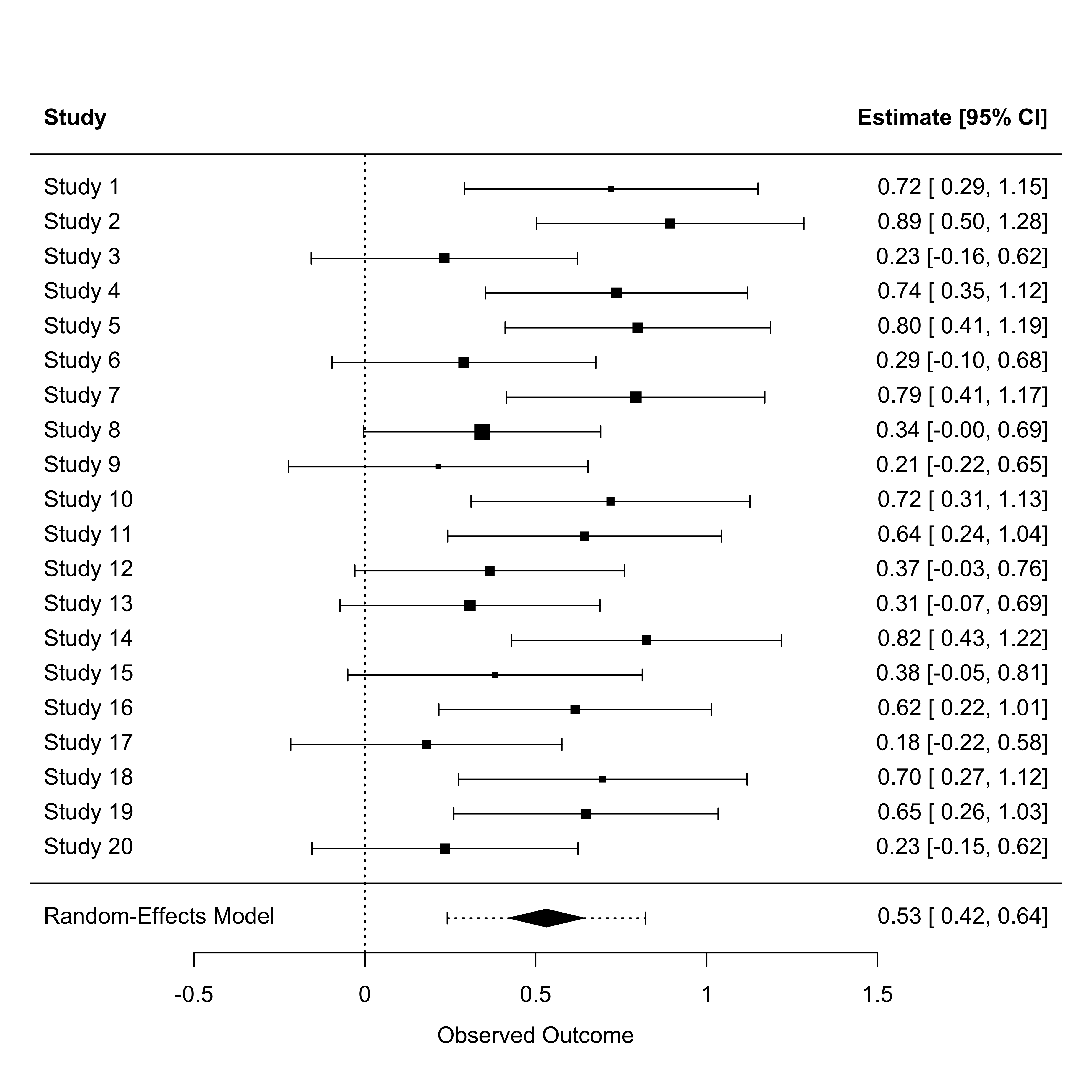
Visualization
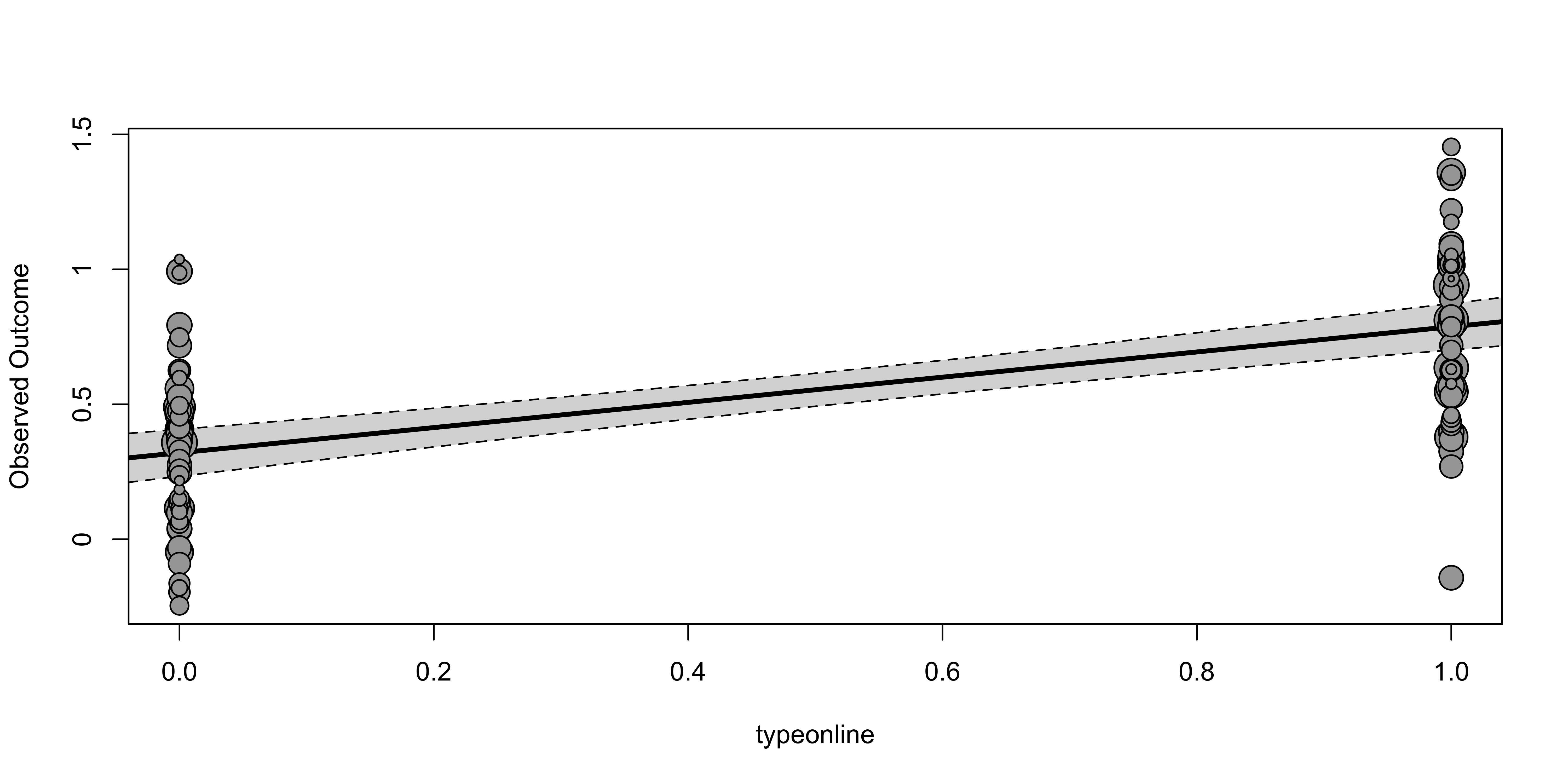
The slope of the regression line visually represents \(\hat{\beta}_1\): the estimated difference in effect size between online and lab-based studies. The circle size reflects inverse-variance weights.
Beyond testing individual coefficients, we can test any linear combination of parameters, for example, whether both lab and online effects are simultaneously different from 0. This is equivalent to fitting a model without the intercept (~ 0 + type), which directly estimates the cell means
Mixed-Effects Model (k = 100; tau^2 estimator: REML)

tau^2 (estimated amount of residual heterogeneity):     0.0286 (SE = 0.0137)
tau (square root of estimated tau^2 value):             0.1691
I^2 (residual heterogeneity / unaccounted variability): 29.73%
H^2 (unaccounted variability / sampling variability):   1.42

Test for Residual Heterogeneity:
QE(df = 98) = 139.4219, p-val = 0.0038

Test of Moderators (coefficients 1:2):
QM(df = 2) = 372.7652, p-val < .0001

Model Results:

            estimate      se     zval    pval   ci.lb   ci.ub
typelab       0.3202  0.0444   7.2099  <.0001  0.2332  0.4072  ***
typeonline    0.7872  0.0440  17.9104  <.0001  0.7011  0.8734  ***

---
Signif. codes:  0 '***' 0.001 '**' 0.01 '*' 0.05 '.' 0.1 ' ' 1
What differences do you notice?
Another solution is to provide a contrast matrix expressing linear combinations of model parameters to be tested.
In our case we test:
\(\text{lab} = \beta_0 = 0\) and
\(\text{online} = \beta_0 + \beta_1 = 0\).
The matrix formulation is:
\[\begin{pmatrix} 1 & 0 \\ 1 & 1 \end{pmatrix} \begin{pmatrix} \beta_0 \\ \beta_1 \end{pmatrix} = \begin{pmatrix} 0 \\ 0 \end{pmatrix}\]
In R:
C <- rbind(c(1, 0), c(1, 1))
B <- coef(fit)
C %*% B  # same as coef(fit)[1] and coef(fit)[1] + coef(fit)[2]
[,1]
[1,] 0.3202007
[2,] 0.7872488
Hypotheses:
1:              intrcpt = 0
2: intrcpt + typeonline = 0

Results:
   estimate     se    zval   pval
1:   0.3202 0.0444  7.2099 <.0001 ***
2:   0.7872 0.0440 17.9104 <.0001 ***

Omnibus Test of Hypotheses:
QM(df = 2) = 372.7652, p-val < .0001
It is important to realize that this does not test whether there are differences between the different forms of experiments (this is what we tested earlier in the model that included the intercept term). However, we can again use contrasts of the model coefficients to test differences between the levels:
Hypotheses:
1: -typelab + typeonline = 0
2:               typelab = 0
3:            typeonline = 0

Results:
   estimate     se    zval   pval
1:   0.4670 0.0625  7.4746 <.0001 ***
2:   0.3202 0.0444  7.2099 <.0001 ***
3: 0.7872 0.0440 17.9104 <.0001 *** Publication Bias
Publication Bias (PB)
Studies included in the meta-analysis differ systematically from all studies that should have been included (Borenstein et al. 2009)
Typically, studies with larger than average effects are more likely to be published, and this can lead to an upward bias in the summary effect (Zwet and Cator 2021)
Small-Study Effects (Borenstein et al. 2009, cap. 30)
We cannot (completely) solve the PB using statistical tools. The PB is a problem related to the publishing process and publishing incentives:
pre-registrations, multi-lab studies, etc. can (almost) completely solve the problem filling the literature with unbiased studies
there are statistical tools to detect, estimate and correct for the publication bias. As every statistical method, they are influenced by statistical assumptions, number of studies and sample size, heterogeneity, etc.
PB under an EE model
The easiest way to understand the PB is by simulating what happen without the PB. Let’s simulate a lot of studies (under a EE model) keeping all the results without selection (the ideal world).
set.seed(2026)
k <- 200
n <- round(runif(k, 10, 100))
theta <- 0.3
dat <- sim_studies(k = k, es = theta, tau2 = 0, n1 = n)
dat <- summary(dat)
head(dat)
  id     yi     vi n1 n2    sei     zi   pval   ci.lb  ci.ub
1  1 0.3343 0.0256 73 73 0.1599 2.0907 0.0366  0.0209 0.6476
2  2 0.2187 0.0307 60 60 0.1751 1.2487 0.2118 -0.1246 0.5619
3  3 0.2195 0.1045 23 23 0.3233 0.6790 0.4971 -0.4141 0.8531
4  4 0.4117 0.0765 36 36 0.2767 1.4880 0.1368 -0.1306 0.9539
5  5 0.2630 0.0302 60 60 0.1738 1.5126 0.1304 -0.0778 0.6037
6 6 0.5445 0.1194 12 12 0.3455 1.5761 0.1150 -0.1326 1.2216 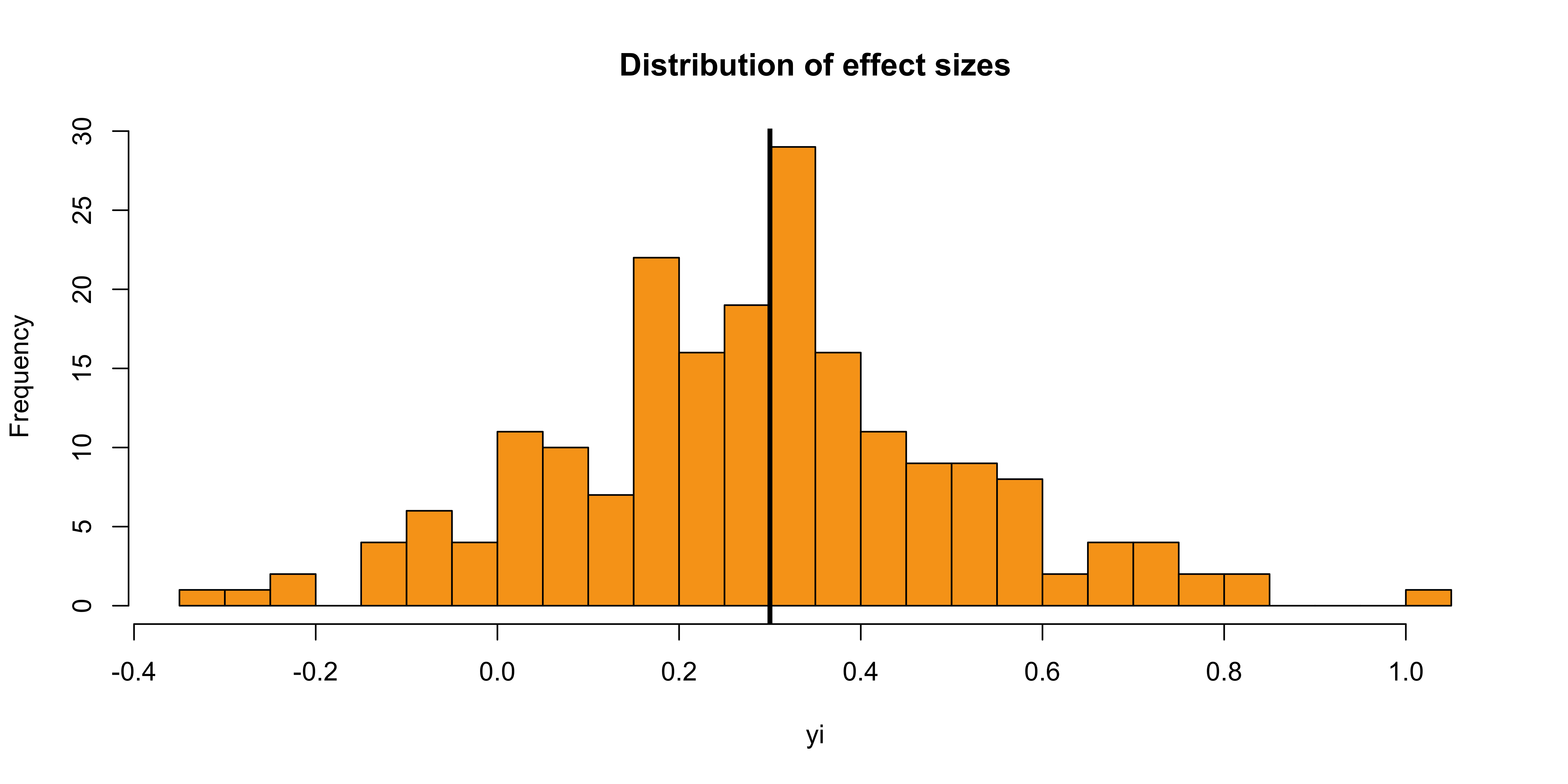
Assuming to pick a very precise and a very unprecise study, which one is more likely to have an effect size close to the true value?
The precise study has a lower \(\epsilon\) thus is closer to \(\theta\). This relationship create a very insightful visual representation.
What could be the shape of the plot when plotting the sampling variances as a function of the effect size?
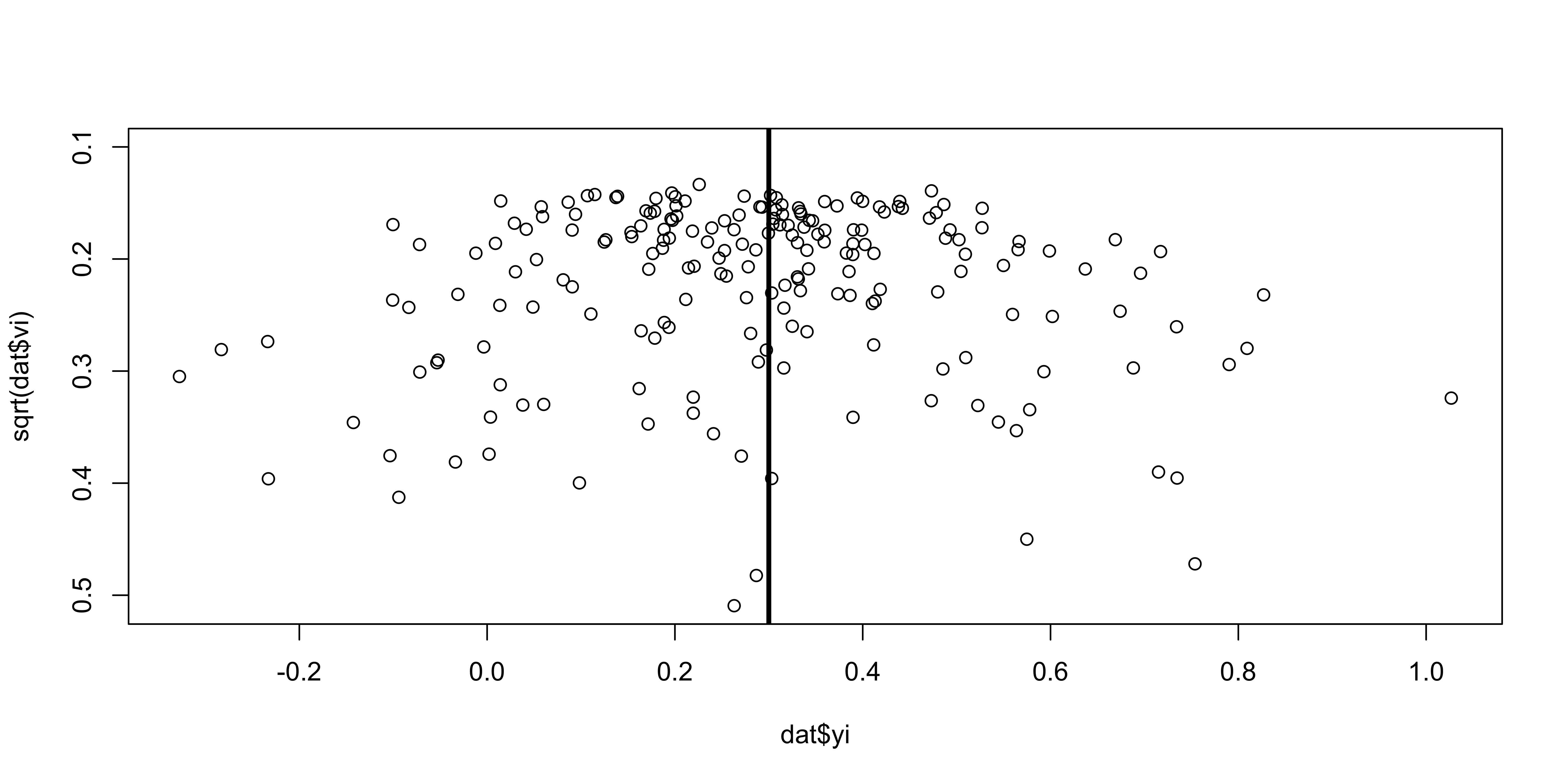
Funnel plot
This is a visual tool to check the presence of asymmetry that could be caused by publication bias. If meta-analysis assumptions are respected, and there is no publication bias:
effects should be normally distributed around the average effect
more precise studies should be closer to the average effect
less precise studies could be equally distributed around the average effect
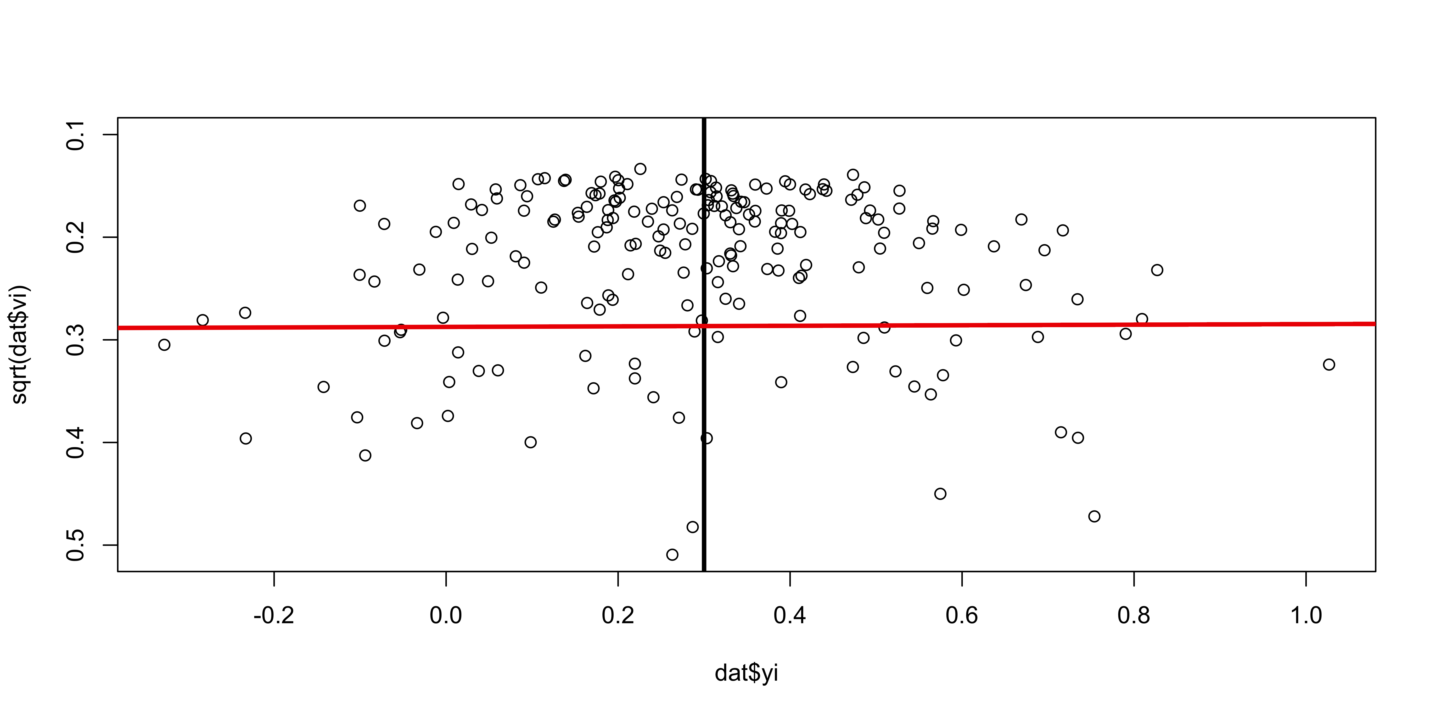
Detecting PB - Egger regression
The plot assume the typical funnel shape and there are not missing spots. The presence of missing spots is a potential index of publication bias.
A basic method to test the funnel plot asymmetry is using an the Egger regression test. Basically we calculate the relationship between \(y_i\) and \(\sqrt{\sigma_i^2}\). In the absence of asimmetry, the line slope should be not different from 0.
Fit EE model
We can use the metafor::regtest() function:
Regression Test for Funnel Plot Asymmetry

Model:     fixed-effects meta-regression model
Predictor: standard error

Test for Funnel Plot Asymmetry: z = 0.2727, p = 0.7851
Limit Estimate (as sei -> 0):   b = 0.2717 (CI: 0.1701, 0.3734)
This is a standard (meta) regression thus the number of studies, the precision of each study and heterogeneity influence the reliability (power, type-1 error rate, etc.) of the procedure.
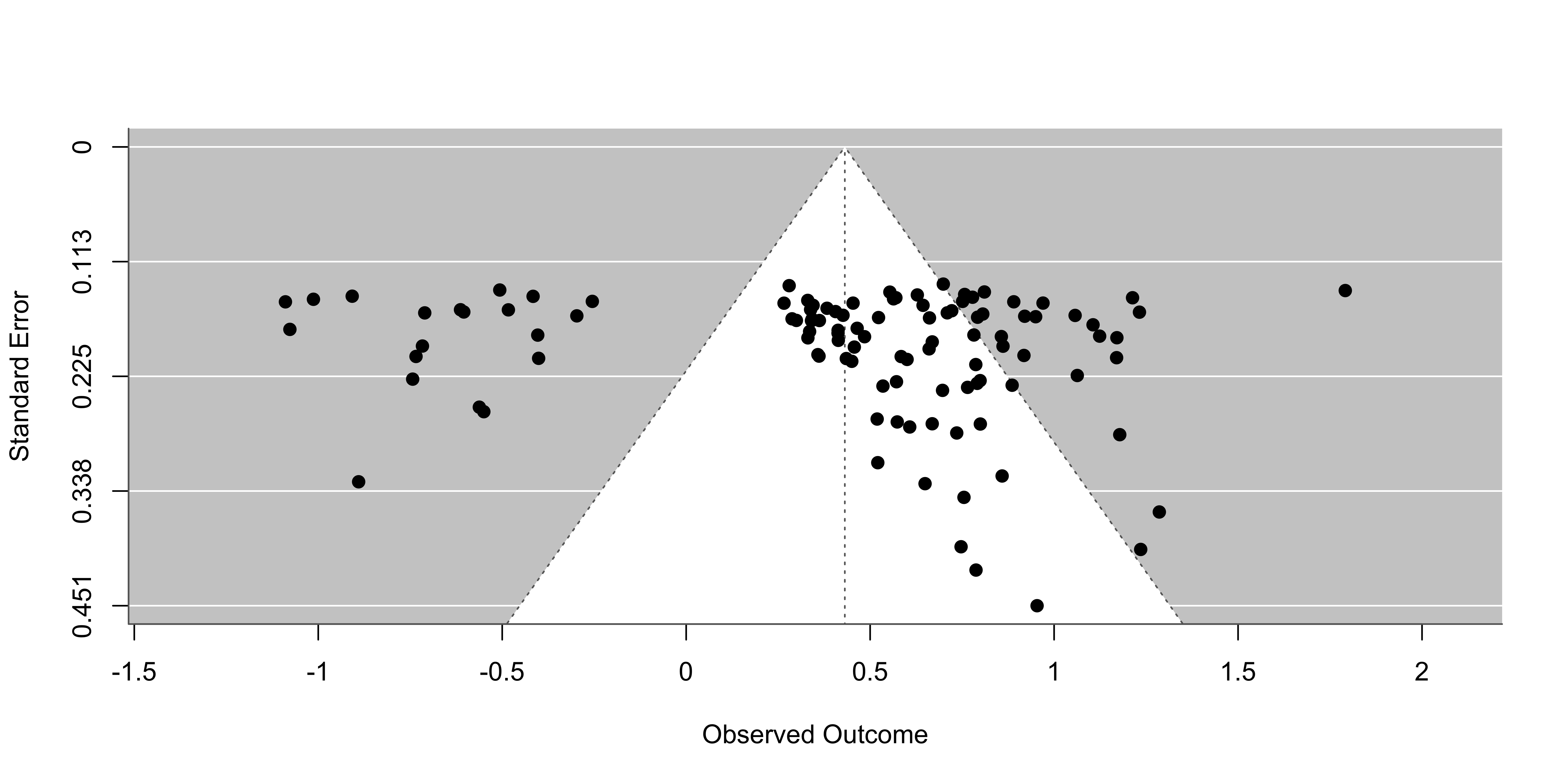
Correcting PB - Trim and Fill
The Trim and Fill method (Duval and Tweedie 2000) is used to impute the hypothetical missing studies according to the funnel plot and recomputing the meta-analysis effect.
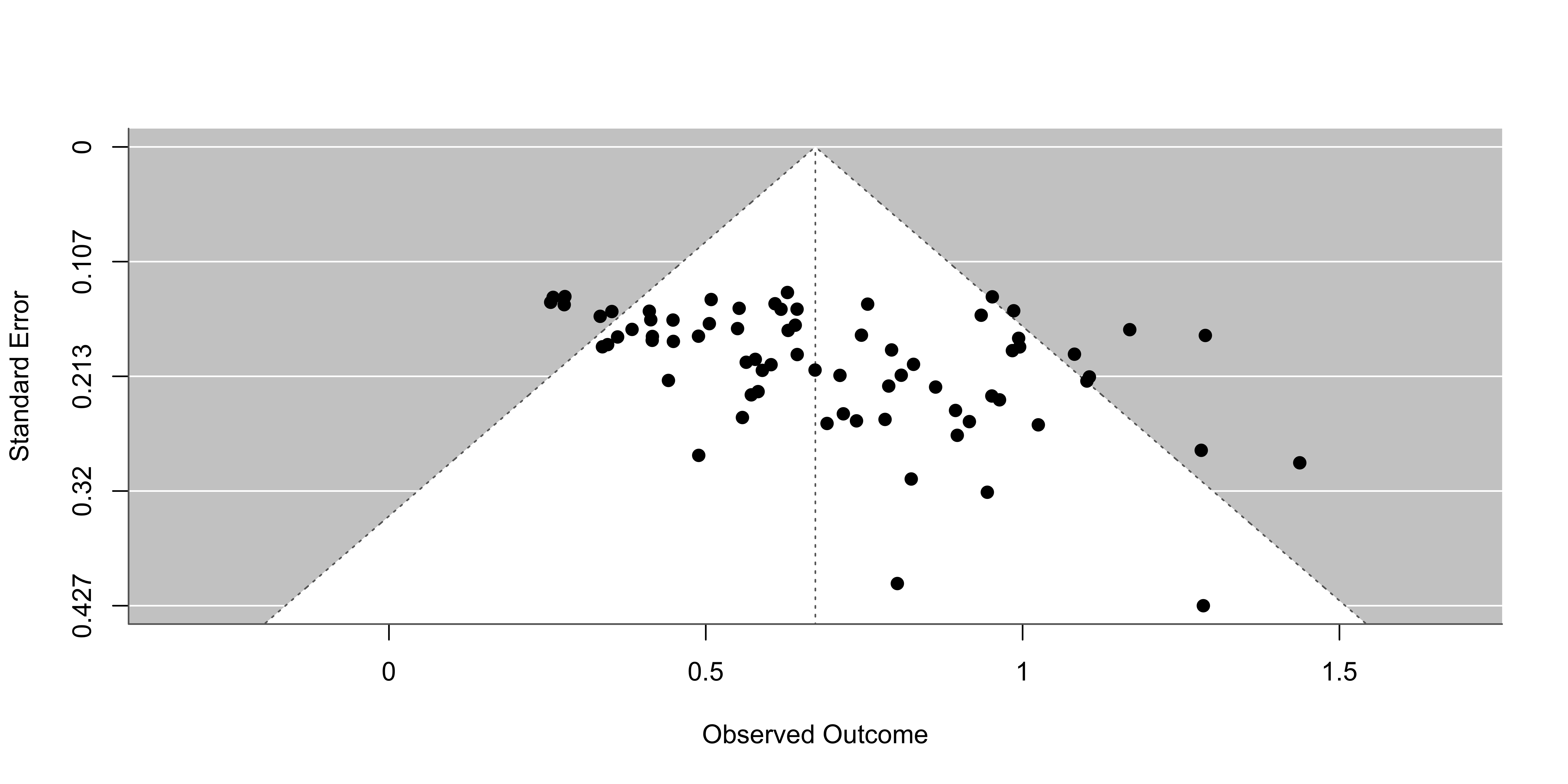
Steps:
estimate the number of studies in the outlying part of the funnel plot;
remove (trim) these studies and do meta-analysis on the remaining studies;
consider the estimate from the “trimmed” meta-analysis as the true center of the funnel;
for each “trimmed” study, create (“fill”) an additional study as the mirror image about the center of funnel plot;
do meta-analysis on the original and filled studies.
(add studies to the funnel plot until it becomes symmetric)
From Rücker, Carpenter, and Schwarzer (2011)
Without trim and fill:
Using the metafor::trimfill() function:
Estimated number of missing studies on the left side: 24 (SE = 5.4307)

Random-Effects Model (k = 97; tau^2 estimator: REML)

tau^2 (estimated amount of total heterogeneity): 0.0973 (SE = 0.0200)
tau (square root of estimated tau^2 value):      0.3119
I^2 (total heterogeneity / total variability):   72.68%
H^2 (total variability / sampling variability):  3.66

Test for Heterogeneity:
Q(df = 96) = 338.7230, p-val < .0001

Model Results:

estimate      se     zval    pval   ci.lb   ci.ub
  0.5267  0.0380  13.8482  <.0001  0.4521  0.6012  ***

---
Signif. codes:  0 '***' 0.001 '**' 0.01 '*' 0.05 '.' 0.1 ' ' 1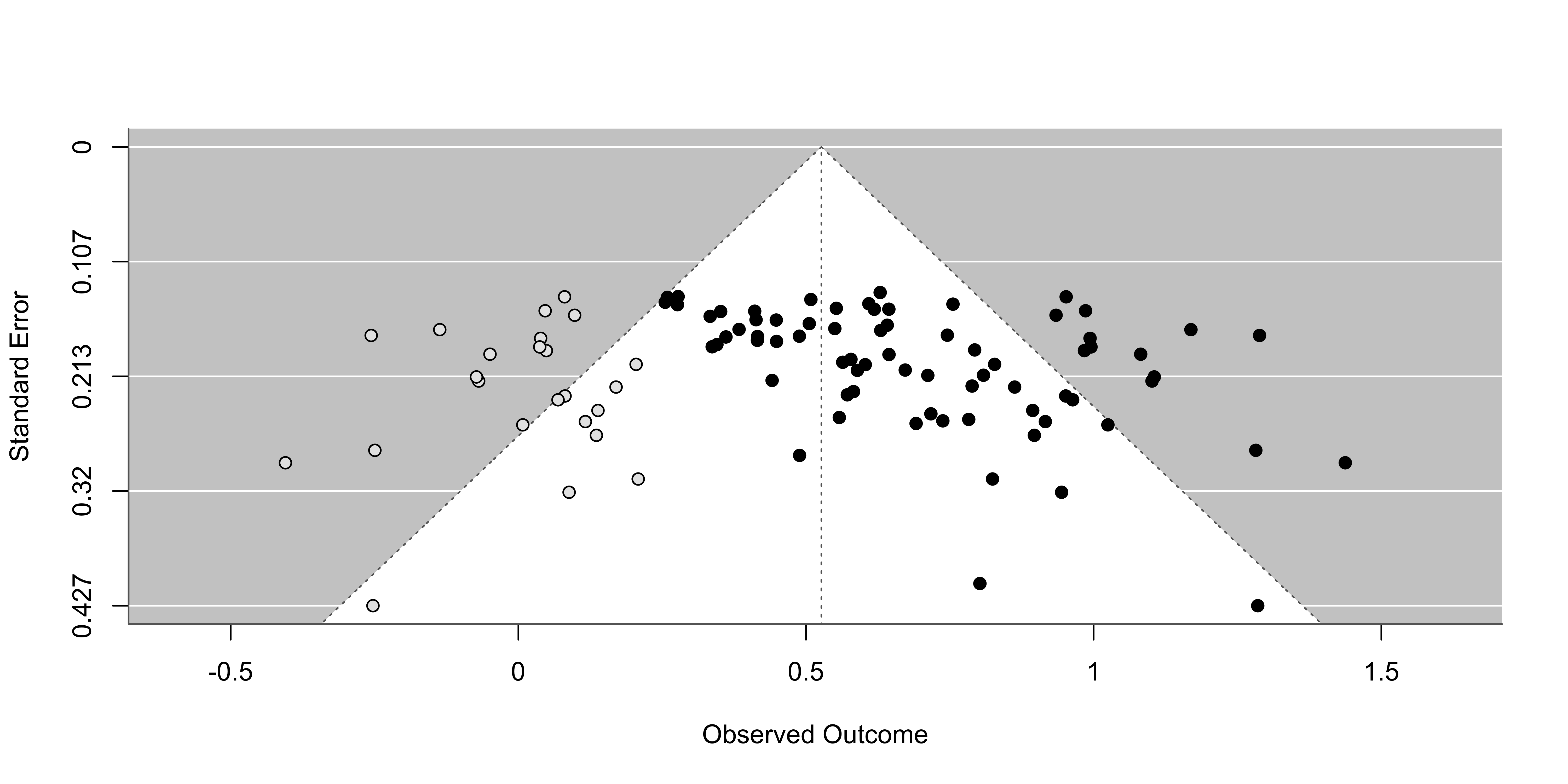
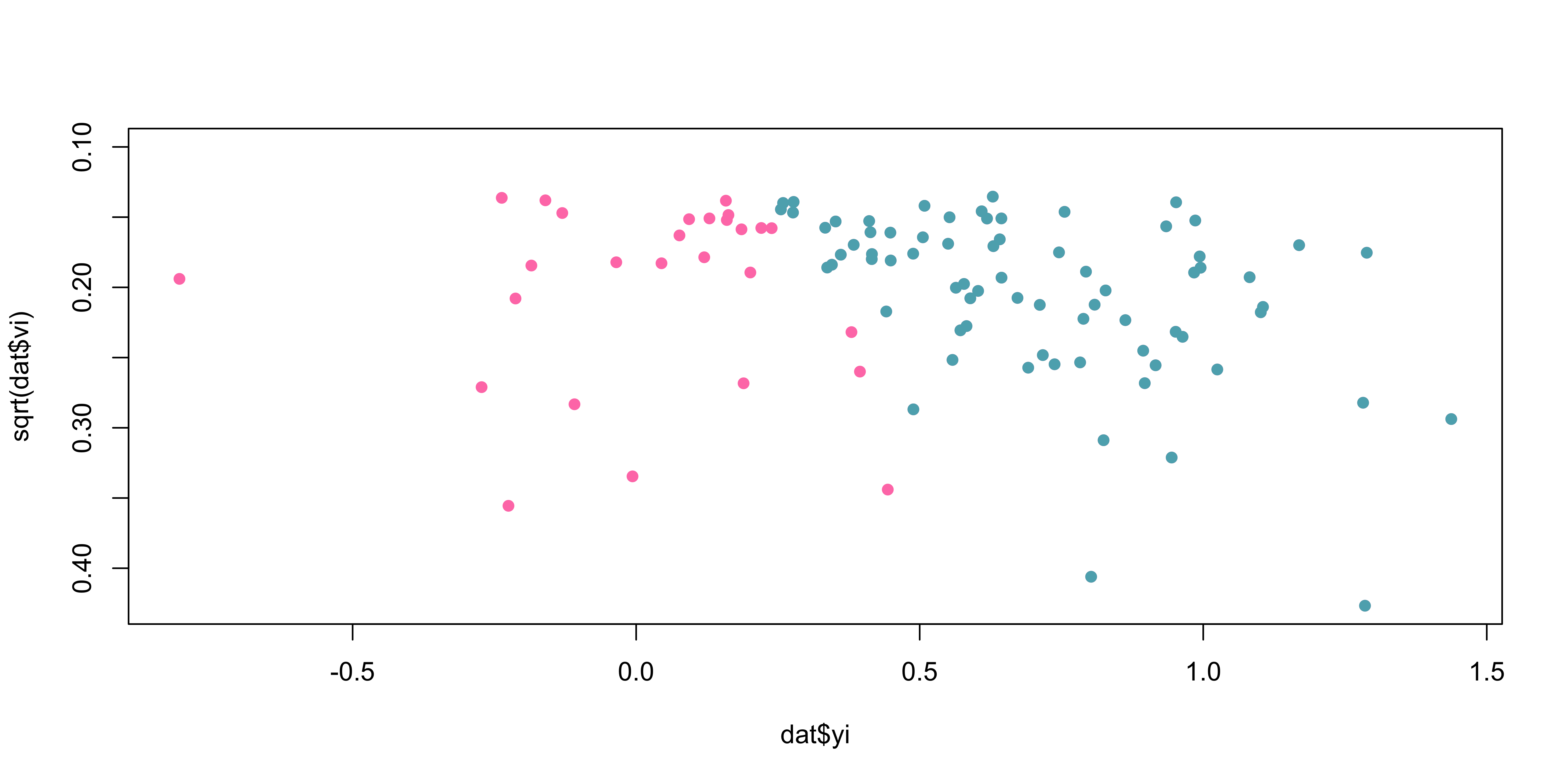
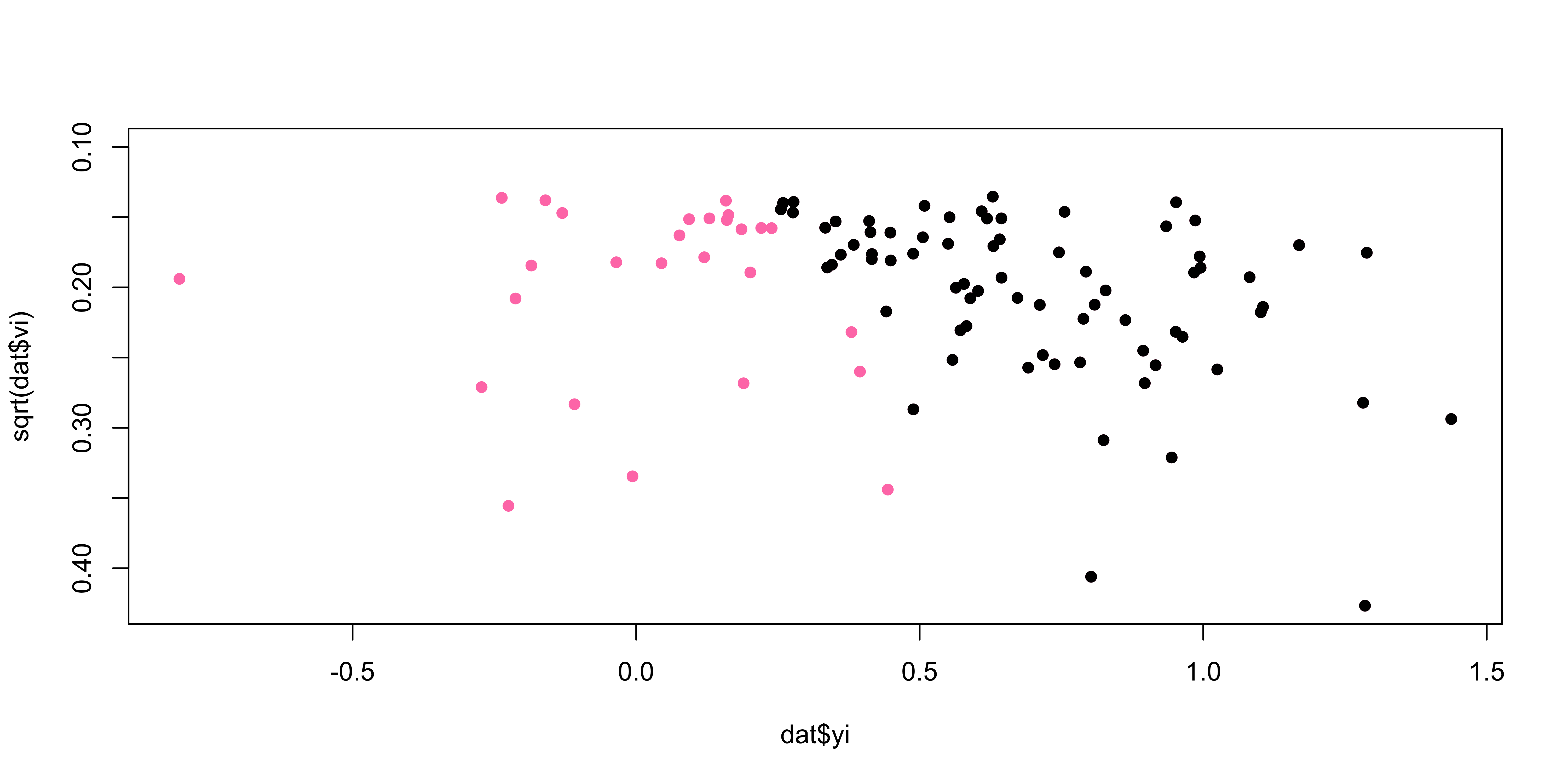
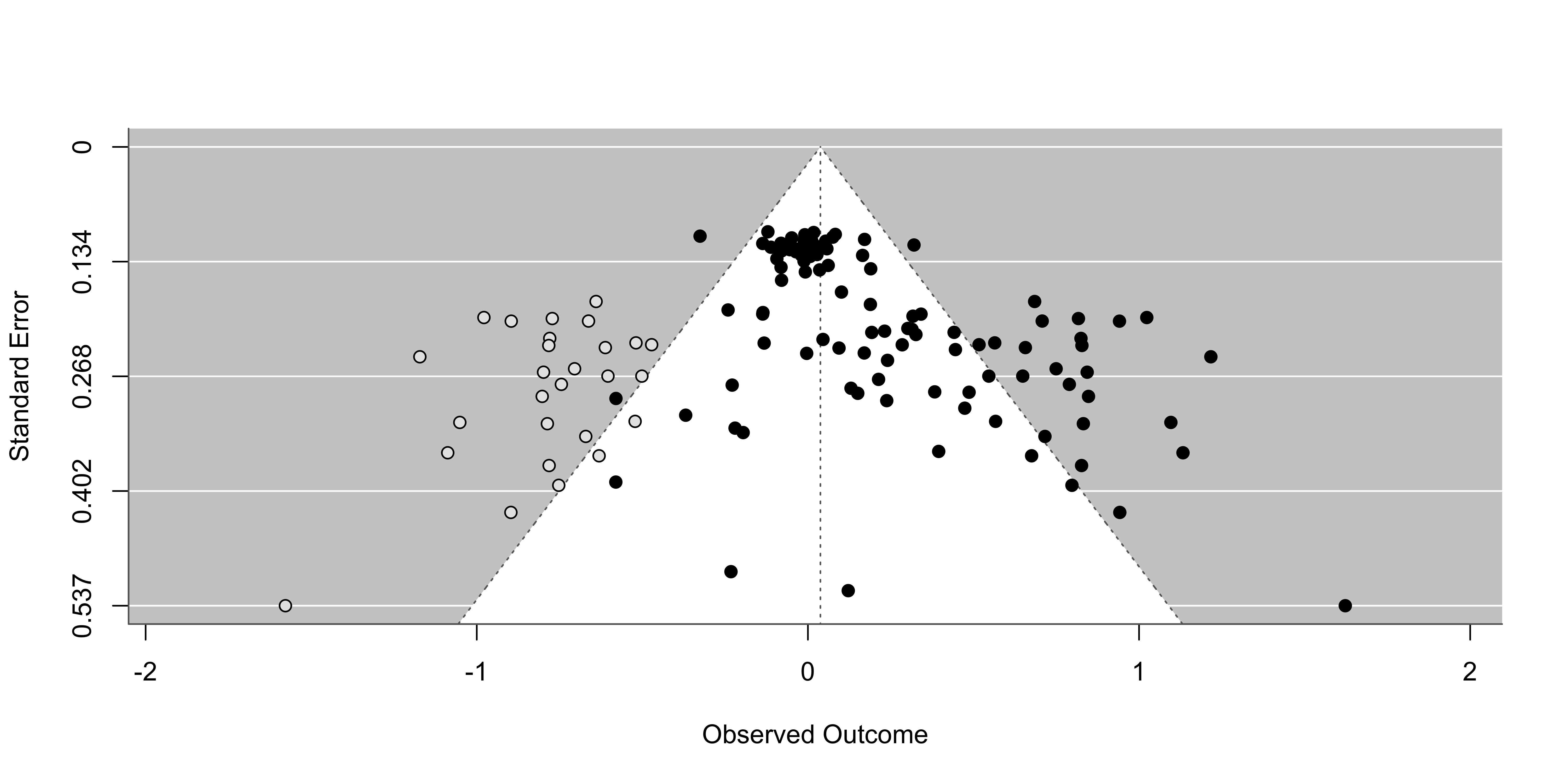
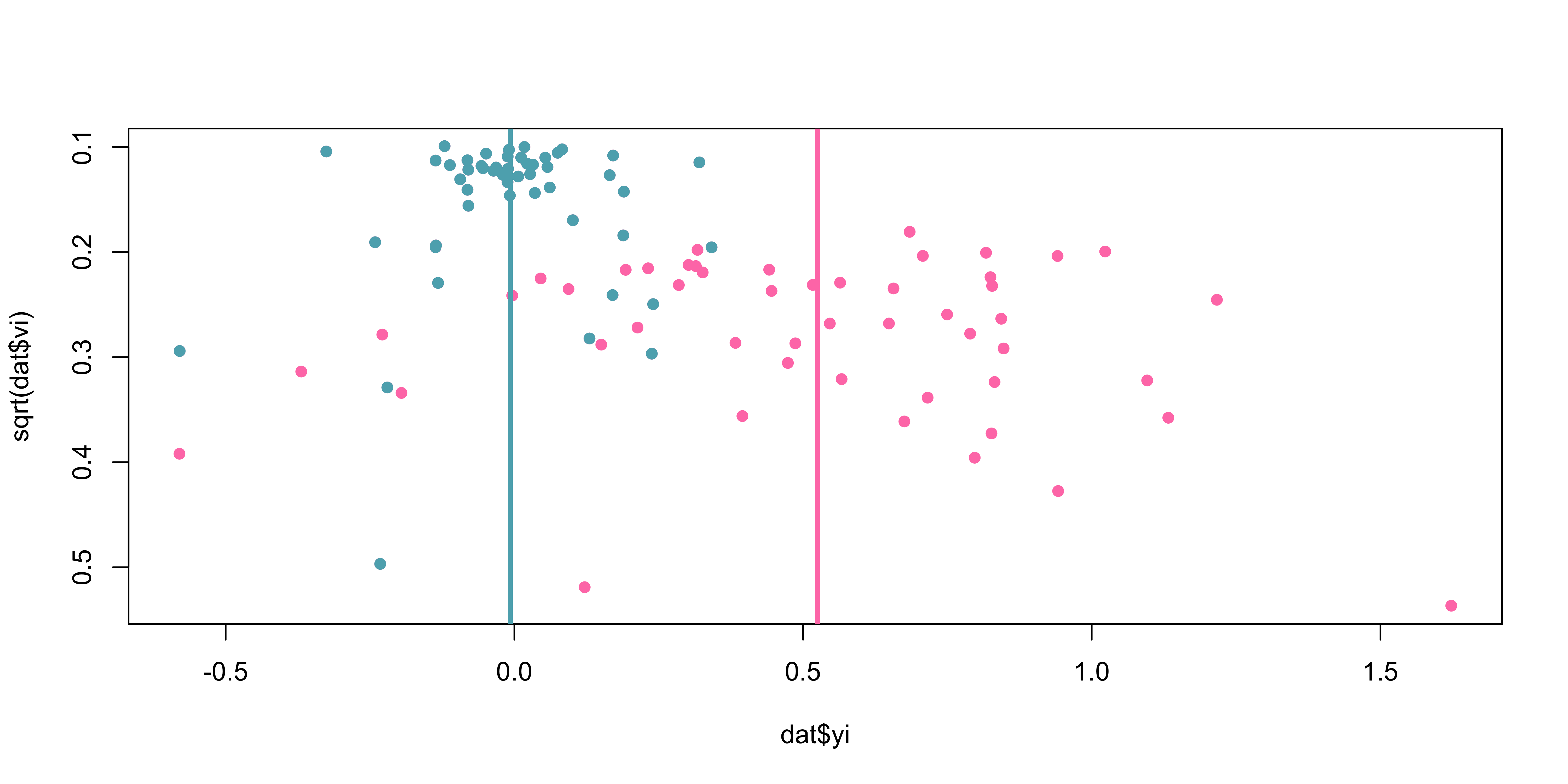
Code
k <- 200
theta <- 0.3
tau2 <- 0.2
n <- round(runif(k, 10, 100))
dat <- sim_studies(k, theta, tau2, n)
dat <- summary(dat)
datpb <- dat[dat$pval <= 0.1, ] # include just studies with small p
plot(dat$yi,sqrt(dat$vi), ylim = c(max(sqrt(dat$vi)), 0.1),
     col = my_cols[1], pch = 16)
points(datpb$yi,sqrt(datpb$vi), pch = 16, col = my_cols[2])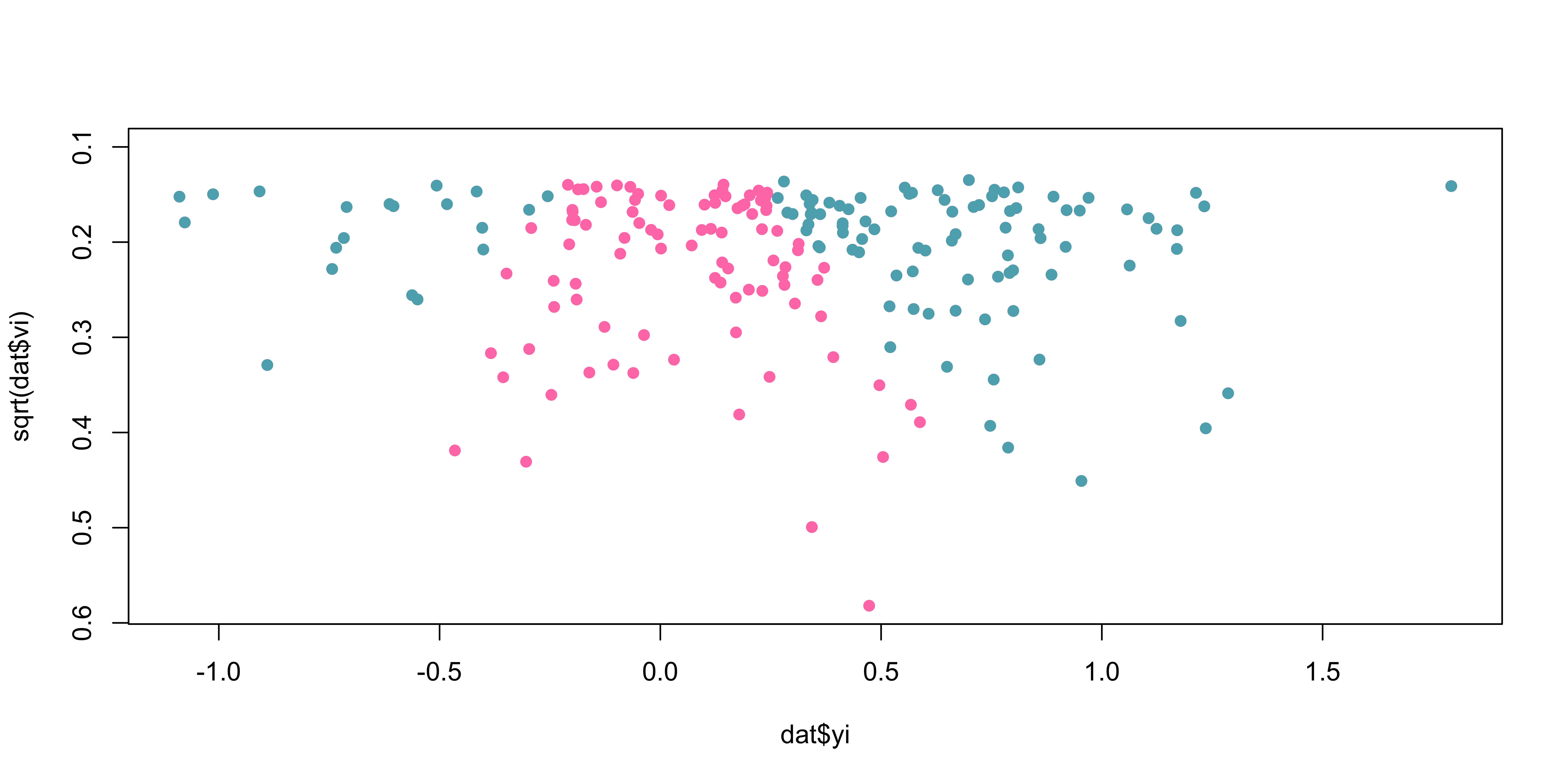
Which studies do you believe have been excluded?
Without trim and fill:
Using the metafor::trimfill() function:
Estimated number of missing studies on the left side: 20 (SE = 6.7941)

Random-Effects Model (k = 127; tau^2 estimator: REML)

tau^2 (estimated amount of total heterogeneity): 0.3893 (SE = 0.0545)
tau (square root of estimated tau^2 value):      0.6239
I^2 (total heterogeneity / total variability):   92.01%
H^2 (total variability / sampling variability):  12.51

Test for Heterogeneity:
Q(df = 126) = 1659.2825, p-val < .0001

Model Results:

estimate      se    zval    pval   ci.lb   ci.ub
  0.2817  0.0584  4.8229  <.0001  0.1672  0.3962  ***

---
Signif. codes:  0 '***' 0.001 '**' 0.01 '*' 0.05 '.' 0.1 ' ' 1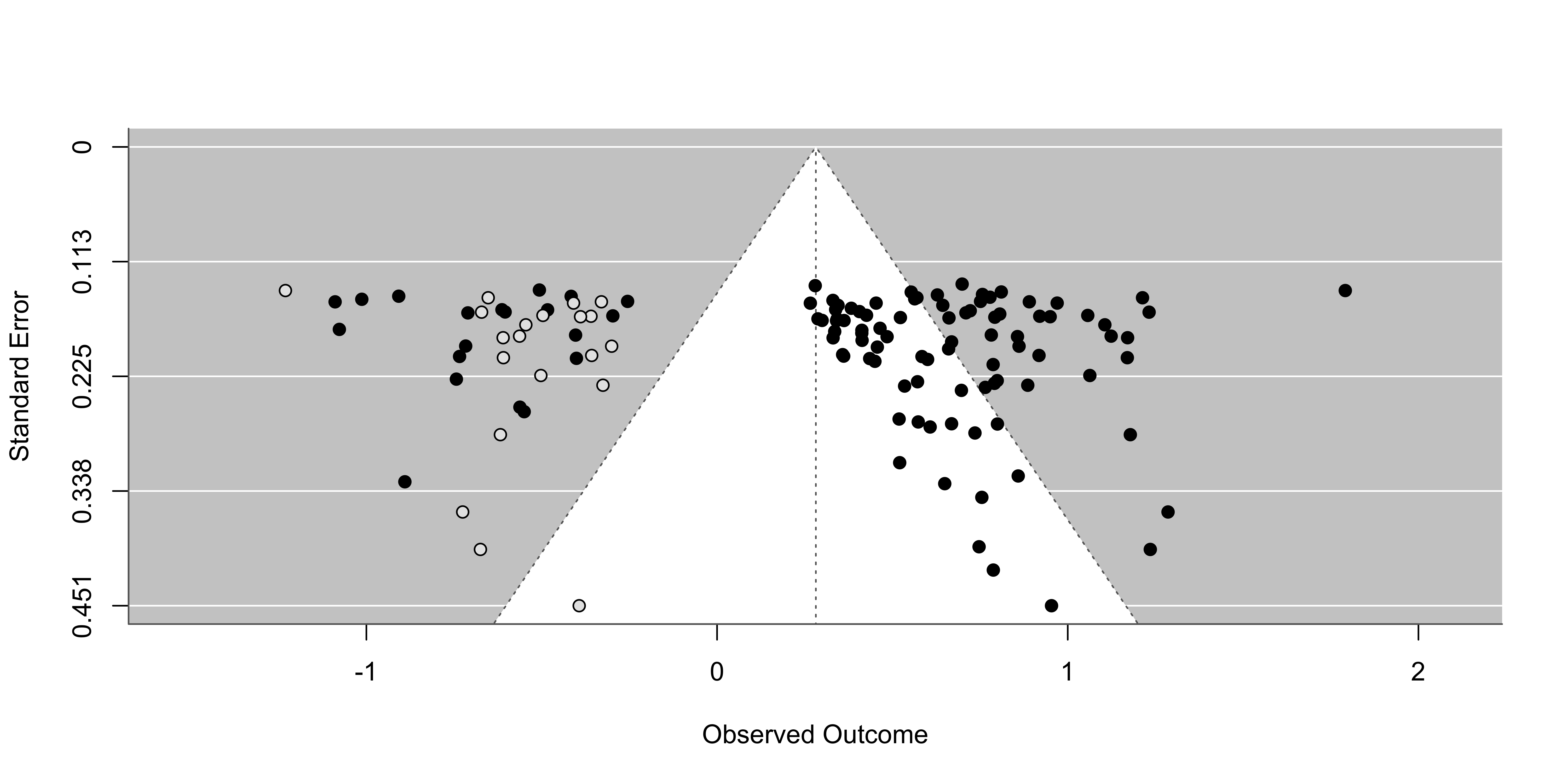

No assumptions about the mechanism leading to publication bias!
Why the funnel plot can be misleading?
Extra source of heterogeneity could create asymmetry not related to PB.
The regtest can be applied also with moderators. The idea should be to take into account the moderators effects and then check for asymmetry.
Beyond funnel plots
Funnel plot asymmetry and trim-and-fill are just two approaches to detecting and correcting for publication bias. Many other methods exist.
Frequentist approaches to PB
A comprehensive overview of available methods is available at: doing-meta.guide/pub-bias
There can be different assumptions about the mechanism generating the bias.
Common pitfalls
Common pitfalls
- Garbage In, Garbage Out: low-quality primaries
- Apples and Oranges: inappropriate aggregation
- Redundant meta-analyses: on some “hot” topics
- Conflicting conclusions: different meta-analyses on the same topic may reach opposite conclusions
- Limited reproducibility: important information is often not reported
Researcher degrees of freedom
Meta-analysis comes with many “researcher degrees of freedom” (Olsson-Collentine et al. 2025; Wicherts et al. 2016), leaving space for decisions which may be arbitrary or reflect undisclosed personal preferences.
Different meta-analyses on overlapping topics often come to different conclusions.
The reproducibility of many meta-analyses is limited because important information is not reported (Lakens, Hilgard, and Staaks 2016).
Modern perspectives
Living meta-analysis: continuously updated as new primary studies become available (e.g., Living SEB Skills Project)
Individual Participant Data (IPD) meta-analysis: uses raw data rather than reported statistics; more flexible and powerful for individual-level moderator analyses.
PIMMA: explores sensitivity to the many analytic choices made during the process (Matteo Manente PhD project :) )
Hierarchy of evidence

Practice in R
The memory training example
We examine the efficacy of memory training on cognitive task performance across studies varying by age group.
| Group | Description |
|---|---|
| Experimental | Receives memory training |
| Control | Receives control treatment |
| Moderator | Age group: adolescents vs. older adults |
Model parameters
| Parameter | Meaning |
|---|---|
| \(\beta_0\) | Baseline effect size (adolescents, \(X = 0\)) |
| \(\beta_1\) | Increment for older adults relative to adolescents |
| \(\beta_0 + \beta_1\) | Effect size for older adults |
Effect size: standardized mean difference (\(d\))
Simulation settings
\[\beta_0 = 0.15 \qquad \beta_1 = 0.50 \qquad \tau_r^2 = 0.05 \qquad k = 16 \text{ studies}\]
Exercises
- Simulate the moderator
ageand effect sizesesusing \(\beta_0\), \(\beta_1\) (see Meta-regression section) - Adapt
sim_studies()for standardized mean differences (see Standardized Effect slide) - Simulate \(k = 16\) studies incorporating
ageas a moderator - Fit an EE model (interpret)
- Fit a RE model (interpret, forest plot (
addpred = TRUE), check PB) - Fit a RE meta-regression on
age(forest plot, interpret, check PB)
This presentation draws in part on workshopmaterials on meta-analysis by Filippo Gambarota and Gianmarco Altoè, course slides by Prof. Altoè (A.A. 2024/2025), and resources including Harrer et al. (2021) and the metafor documentation.
Thank you!