Introduction to Meta-Analysis with Application in R

Application in R

Margherita Calderan

2026-04-10

Practice in R

The Memory Training Example

We examine the efficacy of memory training on cognitive task performance across studies varying by age group.

Group	Description
Experimental	Receives memory training
Control	Receives control treatment
Moderator	Age group: adolescents vs. older adults

Model Parameters

Parameter	Meaning
\(\beta_0\)	Baseline effect size (adolescents, \(X = 0\))
\(\beta_1\)	Increment for older adults relative to adolescents
\(\beta_0 + \beta_1\)	Effect size for older adults

Effect size: standardized mean difference (\(d\))

Simulation Settings

\[\beta_0 = 0.15 \qquad \beta_1 = 0.50 \qquad \tau_r^2 = 0.05 \qquad k = 16 \text{ studies}\]

Exercises

Simulate the moderator age and effect sizes es using \(\beta_0\), \(\beta_1\) (see Meta-regression section)
Adapt sim_studies() for standardized mean differences (see Standardized Effect slide)
Simulate \(k = 16\) studies incorporating age as a moderator
Fit an EE model (interpret)
Fit a RE model (forest plot (addpred = TRUE), interpret, check PB)
Fit a RE meta-regression on age (forest plot, interpret, check PB)

1. Simulate effect sizes `es`

set.seed(1604)

k <- 16
b0 <- 0.15
b1 <- 0.5
  
age <- factor(rep(c("adol", "adult"), each = k/2)) # 100 studies
age_dummy <- ifelse(age == "adol", 0, 1)  # treatment coding

es <- b0 + b1 * age_dummy

2. Adapt `sim_studies()` for standardized mean differences

sim_studies <- function(k, es, tau2 = 0, n1, n2 = NULL, add = NULL){
  if(length(n1) == 1) n1 <- rep(n1, k)
  if(is.null(n2)) n2 <- n1
  if(length(es) == 1) es <- rep(es, k)
  
  yi <- rep(NA, k)
  vi <- rep(NA, k)
  
  # random effects
  deltai <- rnorm(k, 0, sqrt(tau2))
  
  for(i in 1:k){
    g1 <- rnorm(n1[i], 0, 1)
    g2 <- rnorm(n2[i], es[i] + deltai[i], 1)
    v1 <- var(g1)
    v2 <- var(g2)
    
    # pooled standard deviation
    sp <- sqrt(((n1[i]-1)*v1 + (n2[i]-1)*v2) / (n1[i]+n2[i]-2))
    # cohen's d and variance
    yi[i] <- (mean(g2) - mean(g1)) / sp
    vi[i] <- (n1[i] + n2[i])/(n1[i]*n2[i]) + yi[i]^2/(2*(n1[i]+n2[i]))
  }
  
  sim <- data.frame(id = 1:k, yi, vi, n1 = n1, n2 = n2)
  
  if(!is.null(add)){ # we will need this later
    sim <- cbind(sim, add)
  }
  
  # convert to escalc for using metafor
  sim <- metafor::escalc(yi = yi, vi = vi, data = sim)
  
  return(sim)
}

3. Simulate \(k = 16\) studies incorporating `age` as a moderator

tau2r <- 0.05
  
n <- 10 + rpois(k, 30 - 10) # sample sizes

d <- sim_studies(k = k, es = es, n1 = n, 
                 tau2 = tau2r, add = age)

4. Fit an EE Model

fitee <- rma(yi, vi, dat = d, method = "EE")
fitee


Equal-Effects Model (k = 16)

I^2 (total heterogeneity / total variability):   54.15%
H^2 (total variability / sampling variability):  2.18

Test for Heterogeneity:
Q(df = 15) = 32.7143, p-val = 0.0051

Model Results:

estimate      se    zval    pval   ci.lb   ci.ub      
  0.3611  0.0647  5.5822  <.0001  0.2343  0.4878  *** 

---
Signif. codes:  0 '***' 0.001 '**' 0.01 '*' 0.05 '.' 0.1 ' ' 1

4. Fit an EE Model — Interpretation

We fitted an EE model to \(k = 16\) studies. The model assumes a single true effect size shared across all studies, attributing observed variability entirely to sampling error.

Significant heterogeneity detected
54.15% of total variability reflects true between-study differences
2.18, Observed variability is greater than expected from sampling error alone
Pooled Estimate: 0.3611, se = 0.0647

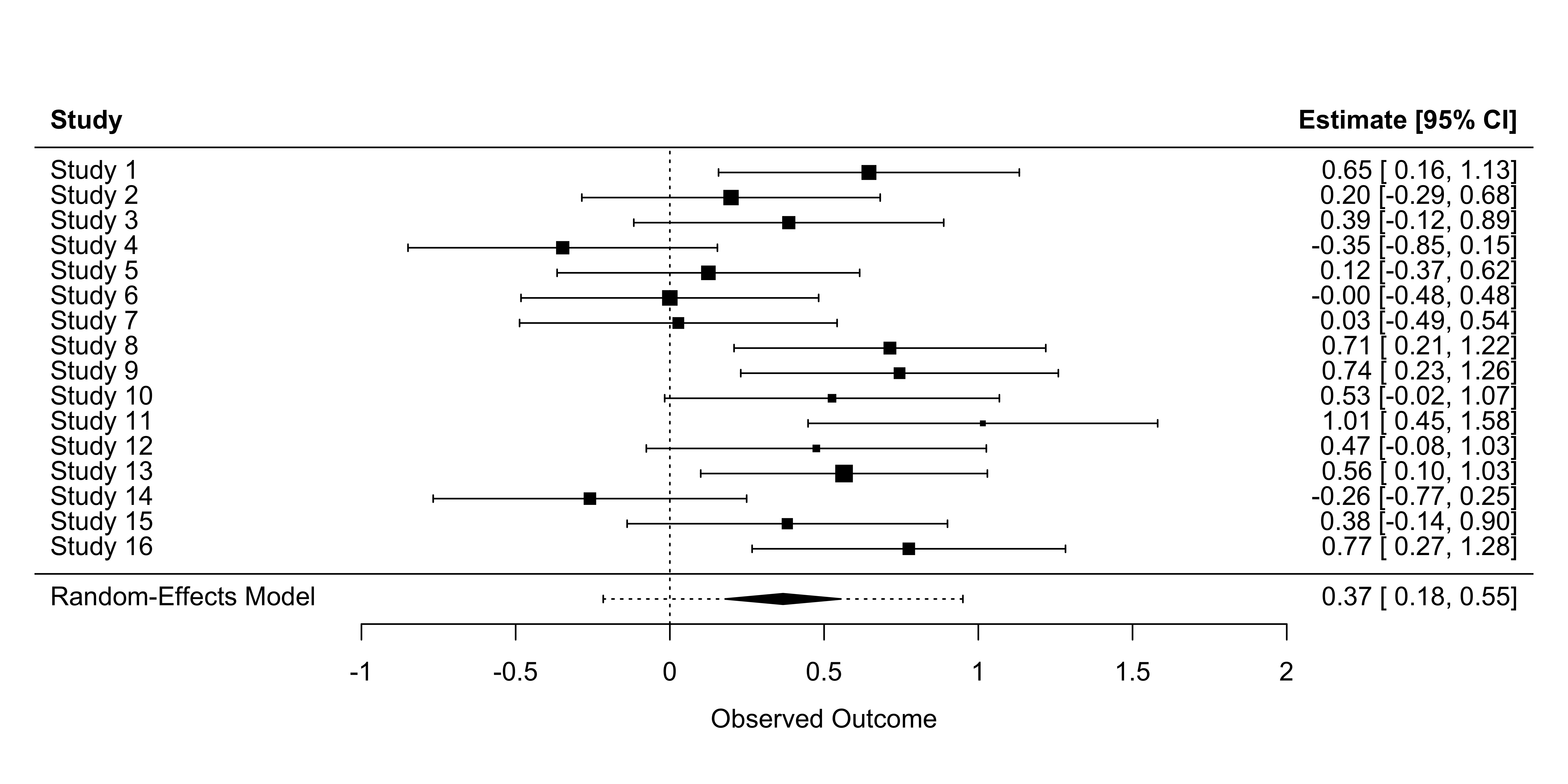
5. Fit a RE model

fitre <- rma(yi, vi, dat = d, method = "REML")
fitre


Random-Effects Model (k = 16; tau^2 estimator: REML)

tau^2 (estimated amount of total heterogeneity): 0.0793 (SE = 0.0535)
tau (square root of estimated tau^2 value):      0.2817
I^2 (total heterogeneity / total variability):   54.22%
H^2 (total variability / sampling variability):  2.18

Test for Heterogeneity:
Q(df = 15) = 32.7143, p-val = 0.0051

Model Results:

estimate      se    zval    pval   ci.lb   ci.ub      
  0.3670  0.0957  3.8334  0.0001  0.1794  0.5546  *** 

---
Signif. codes:  0 '***' 0.001 '**' 0.01 '*' 0.05 '.' 0.1 ' ' 1

5. Interpretation

We fitted a RE model to \(k = 16\) studies using REML estimation. Unlike the EE model, the RE model explicitly accounts for between-study variance \(\tau^2\), assuming effect sizes vary around a mean true effect.

Significant heterogeneity detected
54.15% of total variability reflects true between-study differences
2.18, Observed variability is greater than expected from sampling error alone
0.0793 Estimated between-study variance
Pooled Estimate: 0.3670, se = 0.0957

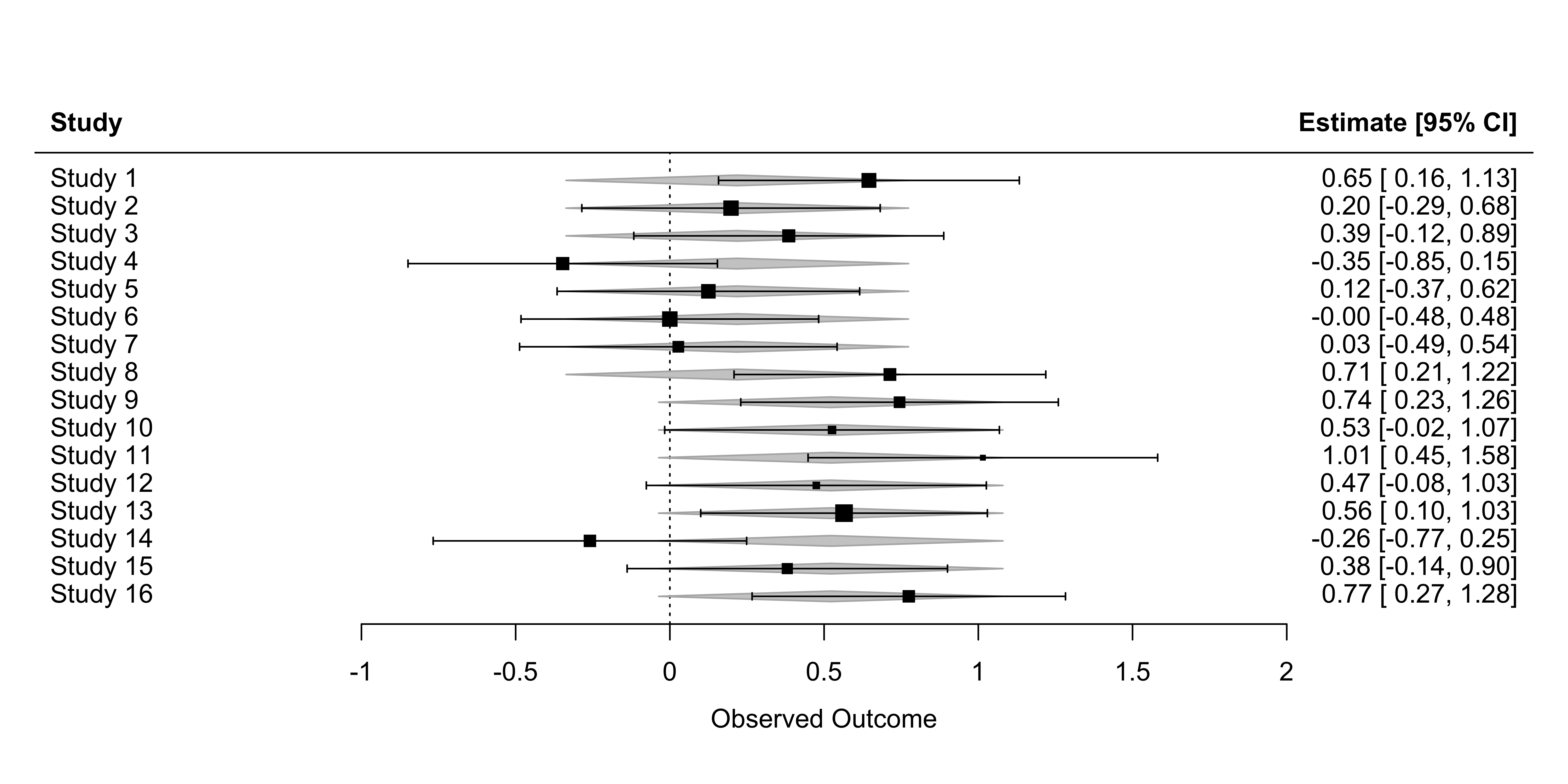
5. Forest plot

forest(fitre, addpred = T)

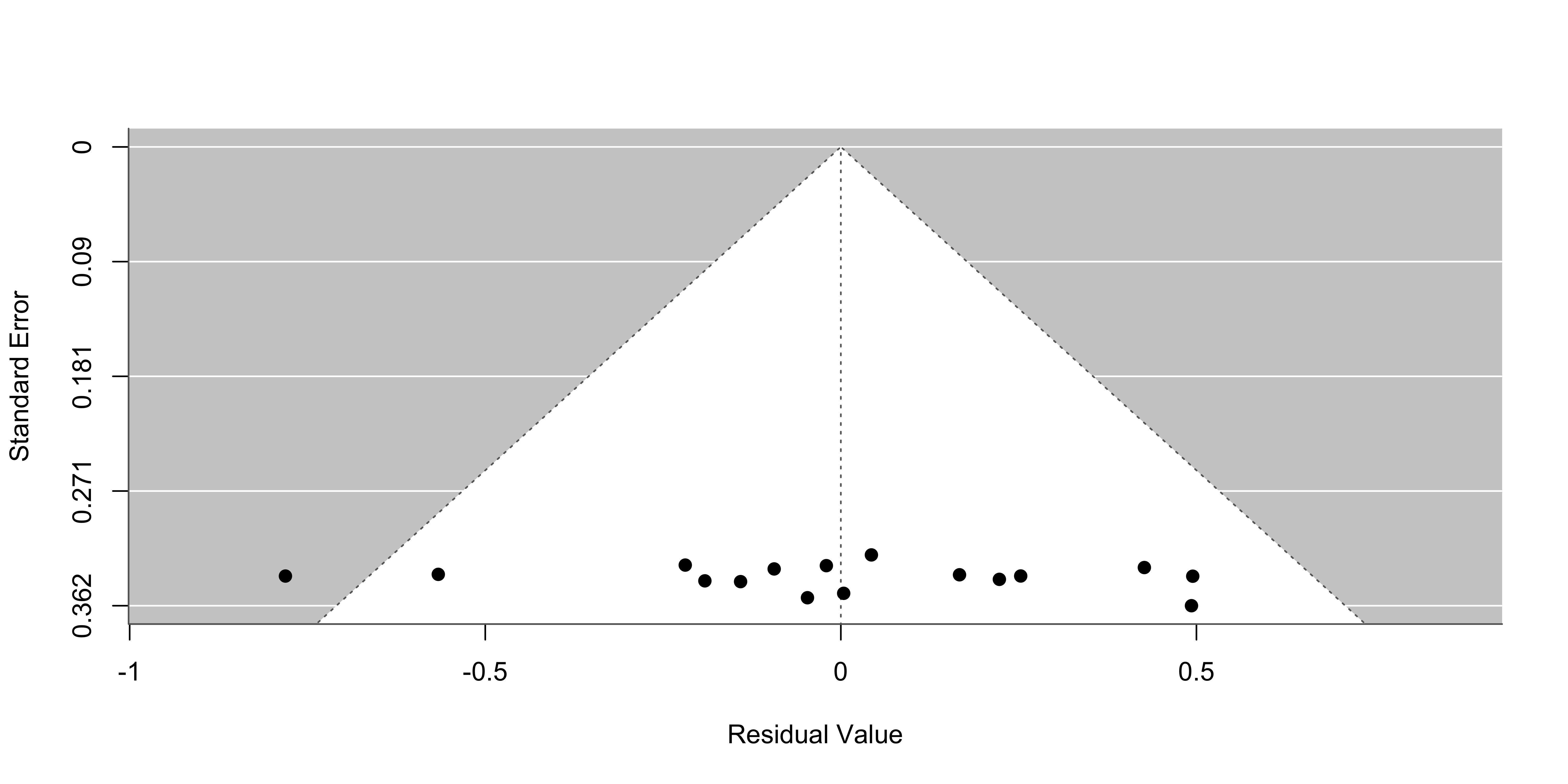
5. Publication bias

funnel(fitre)

regtest(fitre) # no assimetry detected


Regression Test for Funnel Plot Asymmetry

Model:     mixed-effects meta-regression model
Predictor: standard error

Test for Funnel Plot Asymmetry: z =  1.3296, p = 0.1837
Limit Estimate (as sei -> 0):   b = -2.1327 (CI: -5.8219, 1.5565)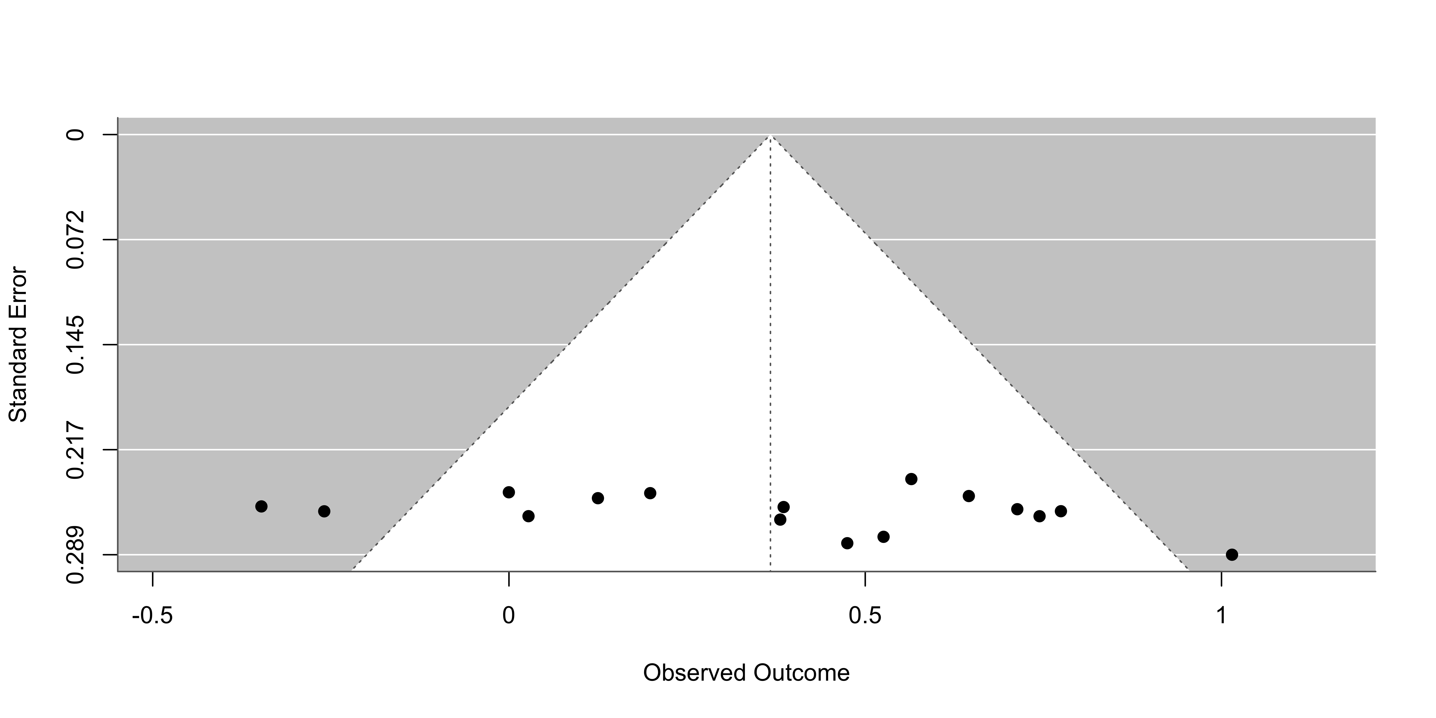

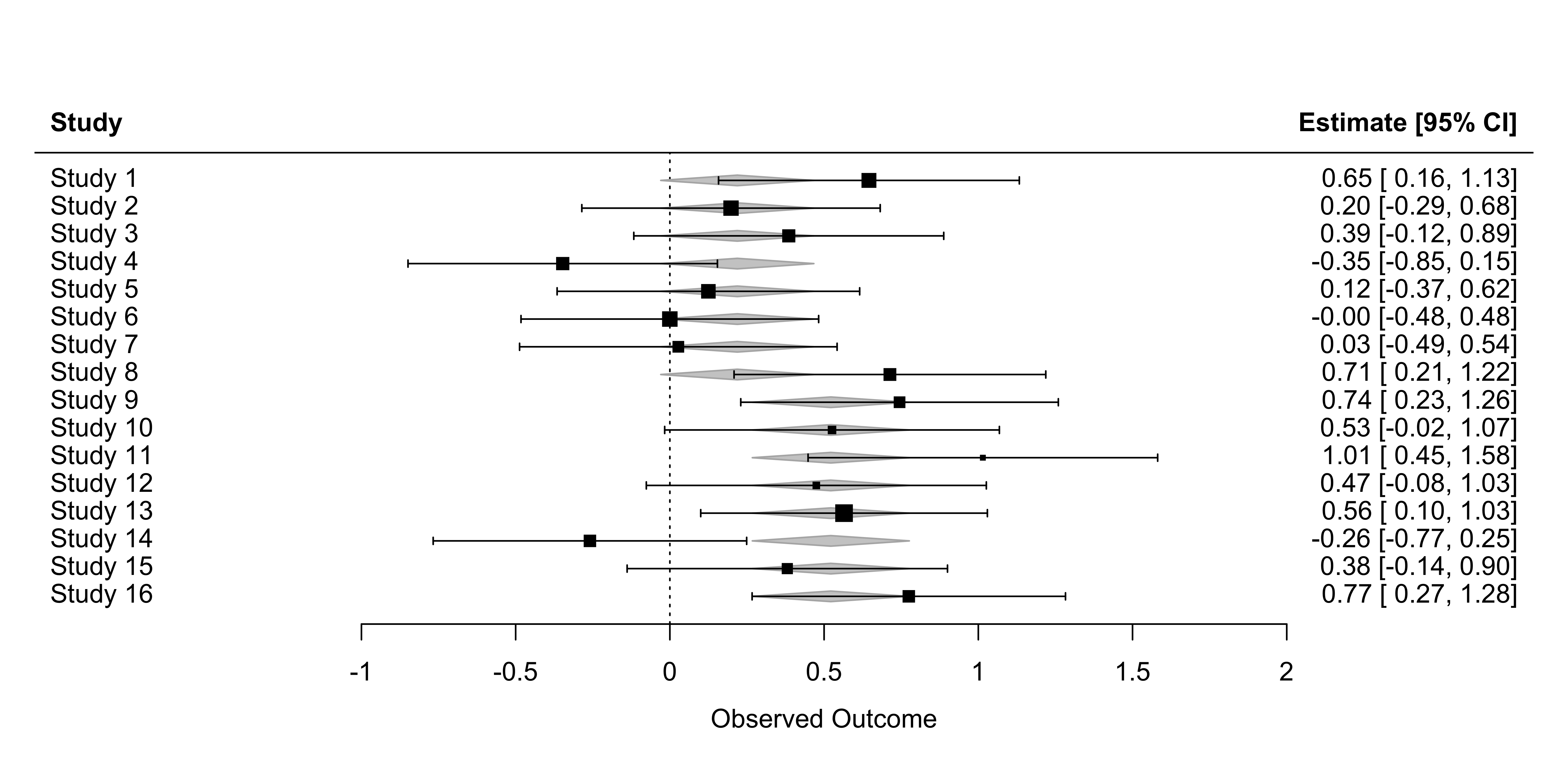
6. Fit a RE-regression model

We extended the RE model by including age group (adolescents vs. older adults) as a moderator, using REML estimation across \(k = 16\) studies.

fitreg <- rma(yi, vi, mods = ~ age, dat = d, method = "REML")
fitreg


Mixed-Effects Model (k = 16; tau^2 estimator: REML)

tau^2 (estimated amount of residual heterogeneity):     0.0642 (SE = 0.0496)
tau (square root of estimated tau^2 value):             0.2534
I^2 (residual heterogeneity / unaccounted variability): 48.93%
H^2 (unaccounted variability / sampling variability):   1.96
R^2 (amount of heterogeneity accounted for):            19.06%

Test for Residual Heterogeneity:
QE(df = 14) = 27.4025, p-val = 0.0171

Test of Moderators (coefficient 2):
QM(df = 1) = 2.7938, p-val = 0.0946

Model Results:

          estimate      se    zval    pval    ci.lb   ci.ub    
intrcpt     0.2186  0.1266  1.7267  0.0842  -0.0295  0.4668  . 
ageadult    0.3031  0.1814  1.6715  0.0946  -0.0523  0.6586  . 

---
Signif. codes:  0 '***' 0.001 '**' 0.01 '*' 0.05 '.' 0.1 ' ' 1

6. Interpretation

We fitted a RE-regression model to \(k = 16\) studies using REML estimation. Unlike the EE model, the RE model explicitly accounts for between-study variance \(\tau^2\), assuming effect sizes vary around a mean true effect.

Significant residual heterogeneity remains after including the moderator
48.93% residual heterogeneity / unaccounted variability
1.96, unaccounted variabilityis greater than expected from sampling error alone
Age group explains 19.06% of the total between-study heterogeneity
0.0642 Residual between-study variance after accounting for age (simulated 0.05)
Age group does not significantly explain between-study variability, p-val = 0.0946

6. Forest plot

forest(fitreg, addpred = F)

6. Forest plot

forest(fitreg, addpred = T)

5. Publication bias

funnel(fitreg)

regtest(fitreg) # no assimetry detected


Regression Test for Funnel Plot Asymmetry

Model:     mixed-effects meta-regression model
Predictor: standard error

Test for Funnel Plot Asymmetry: z = 0.6362, p = 0.5246

Introduction to Meta-Analysis with Application in R

Practice in R

The Memory Training Example

Model Parameters

Simulation Settings

Exercises

1. Simulate effect sizes es

2. Adapt sim_studies() for standardized mean differences

3. Simulate \(k = 16\) studies incorporating age as a moderator

4. Fit an EE Model

4. Fit an EE Model — Interpretation

5. Fit a RE model

5. Interpretation

5. Forest plot

5. Publication bias

6. Fit a RE-regression model

6. Interpretation

6. Forest plot

6. Forest plot

5. Publication bias

1. Simulate effect sizes `es`

2. Adapt `sim_studies()` for standardized mean differences

3. Simulate \(k = 16\) studies incorporating `age` as a moderator