Intro to EAM

@47th ECVP 2025 Mainz

Margherita Calderan

August 24, 2025

Perception into action

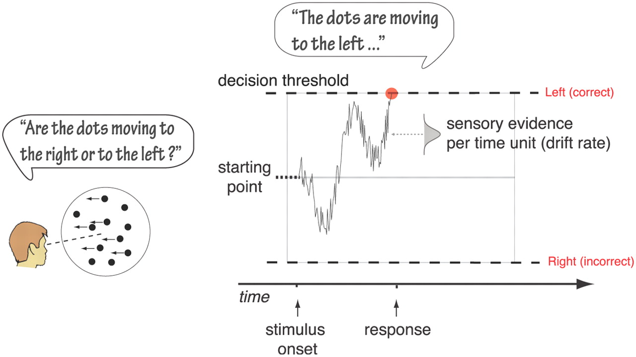
Evidence Accumulation Models assume that, upon stimulus presentation, the decision maker:

• Samples noisy evidence for available options (e.g., “Should I press left or right?”)
• Accumulates that evidence until a threshold is crossed

Mulder, M. J., Wagenmakers, E. J., Ratcliff, R., Boekel, W., & Forstmann, B. U. (2012). Bias in the brain: a diffusion model analysis of prior probability and potential payoff. Journal of Neuroscience, 32(7), 2335–2343.

The brain samples information from the environment, you accumulate that evidence until you’re confident enough to make a decision — say, pressing left or pressing right. Once the accumulated evidence passes a threshold, action is triggered. This is what evidence accumulation models capture.

What is “evidence”?

Neural signals reflecting sensory or internal information relevant to a choice.

“Are dots moving to the right or to the left?”

• Neurons fire in proportion to motion direction & strength.
• These firing rates = momentary evidence.
• Noisy and varies trial-to-trial.

How does the brain accumulate evidence?

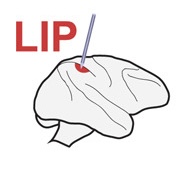
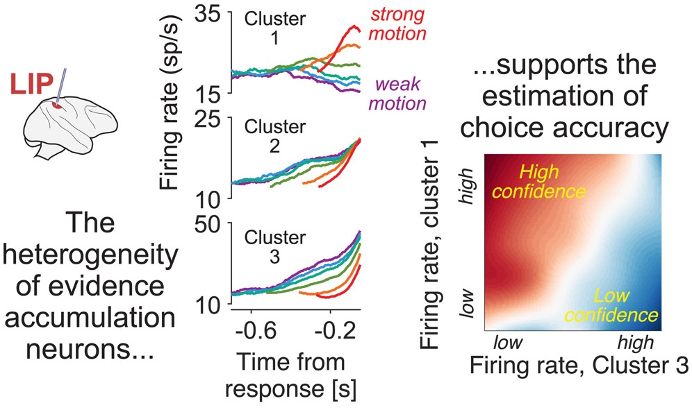
Integrator neurons receive this input

• Neurons in LIP, dlPFC, or striatum ramp up/down over time.

• Reflects accumulated evidence

Zylberberg & Shadlen, 2025

Neurons in the lateral intraparietal (LIP) area with response fields overlapping the choice-target contralateral to the recording site (Tin neurons) represent the accumulation of evidence in favor of contralateral target selection. The monkey reports its decision via a saccadic eye movement to one of the targets and is rewarded for correct choices. In trials where the monkey chooses the contralateral target (i.e., the one within the neurons’ response field), the Tin neurons represent the winning race, whereas on ipsilateral choices, they represent the losing race.

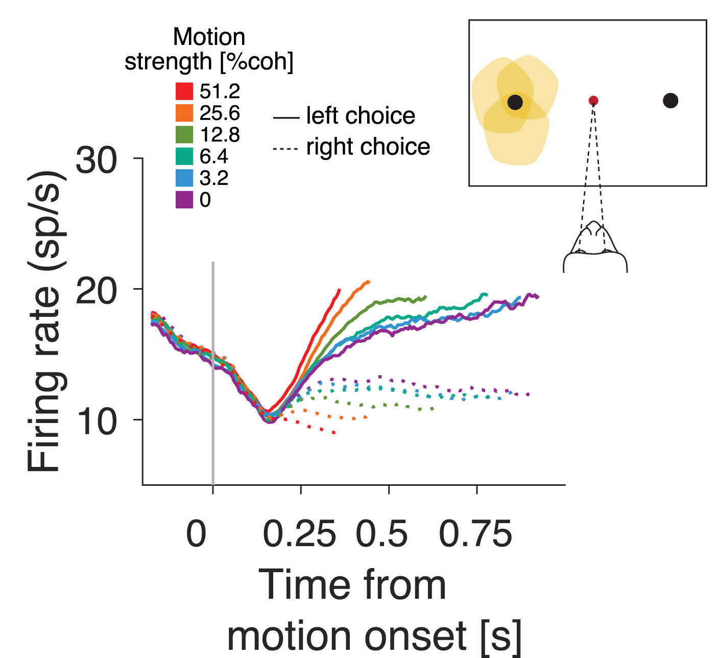
Threshold crossing triggers a decision

Zylberberg & Shadlen, 2025

Brain computation of decisions

Cognitive Term	Neural Interpretation
Evidence	Sensory neuron firing rates
Accumulation	Integration in parietal/frontal areas
Noise	Trial-to-trial neural variability
Bound	Decision threshold in firing/activity

Latent Cognitive Parameters

Sequential processing assumption

Total Response Time (RT) is modeled as the sum of three sequential stages:

1. Stimulus encoding
2. Evidence accumulation (decision-making)
3. Motor response execution

Stages (1) and (3) are captured in the nondecision time (Ter) parameter.

EAMs decompose decisions into:

• Drift rate

• Threshold

Drift Rate

Reflects evidence strength

• ⬆ Drift: fast & accurate decisions

• ⬇ Drift: slow, error-prone

Manipulated by stimulus discriminability/task difficulty

Thresholds

Set before stimulus onset

Reflect response caution/cognitive control/bias/preference

• ⬆ Threshold: Slower but more accurate

• ⬇ Threshold: Faster but error-prone

Manipulate via pre-trial cues or instructions.

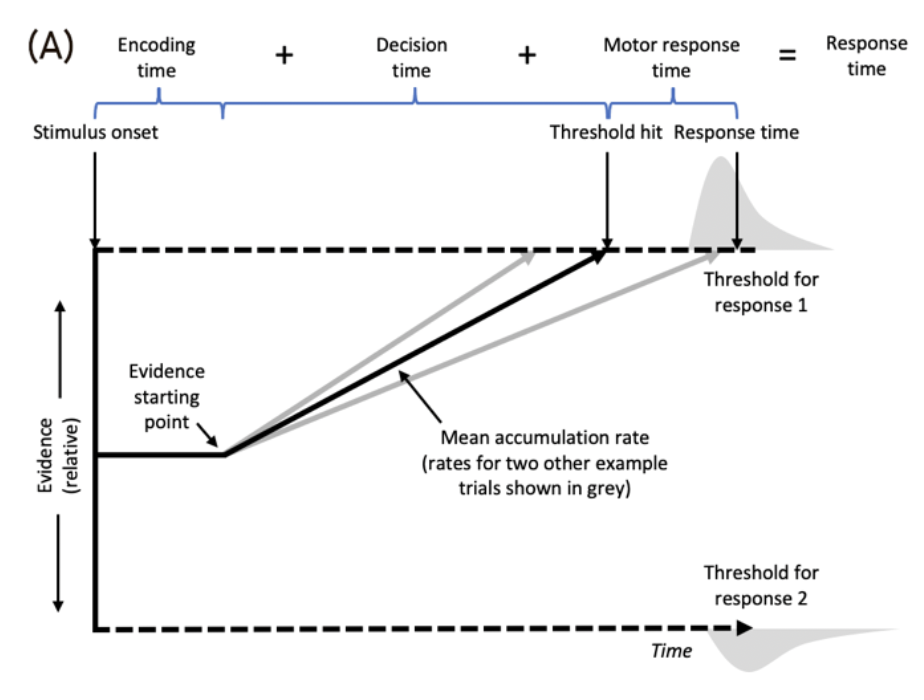
Relative Evidence Models

In relative evidence models (e.g., Wiener process, Diffusion Decision Model):

• Decision is based on the difference in accumulated evidence between two options.

• Suitable for binary choices.

Boag, R. J., Innes, R. J., Stevenson, N., Bahg, G., Busemeyer, J. R., Cox, G. E., … Forstmann, B. (2024, July 2). An expert guide to planning experimental tasks for evidence accumulation modelling.

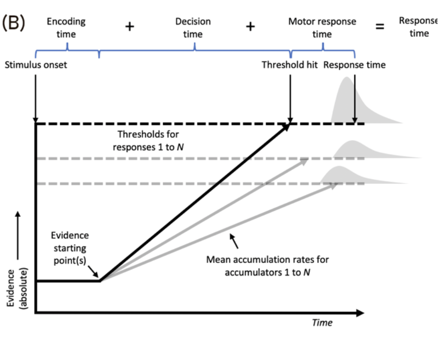
Absolute Evidence Models

In racing accumulator models (e.g., LBA, RDM):

• Each option has its own accumulator tracking absolute evidence.

• Decision is made by the first accumulator to reach threshold.

• Can handle multiple alternatives (not just binary choices).

Boag, R. J., Innes, R. J., Stevenson, N., Bahg, G., Busemeyer, J. R., Cox, G. E., … Forstmann, B. (2025) An expert guide to planning experimental tasks for evidence accumulation modelling.

Although relative and absolute evidence models differ in how they conceptualize evidence, they:

• Share similar assumptions about trial structure and data quality
• Use overlapping parameters (drift rate, threshold, bias, nondecision time)
• Often reach the same substantive conclusions
• Provide convergent results when applied to the same data

Noisy process

Wiener Process

The Wiener process (Brownian motion) is the foundation of many decision models (Smith & Ratcliff, 2024). It models the accumulation of evidence as a noisy process:

$$x(t) = z + vt + sW(t)$$

• $x(t)$: accumulated evidence at time $t$
• z: starting point
• v: drift rate (signal strength)
• s: noise (standard deviation of the increments)
• $W(t)$: standard Wiener process (Gaussian increments)

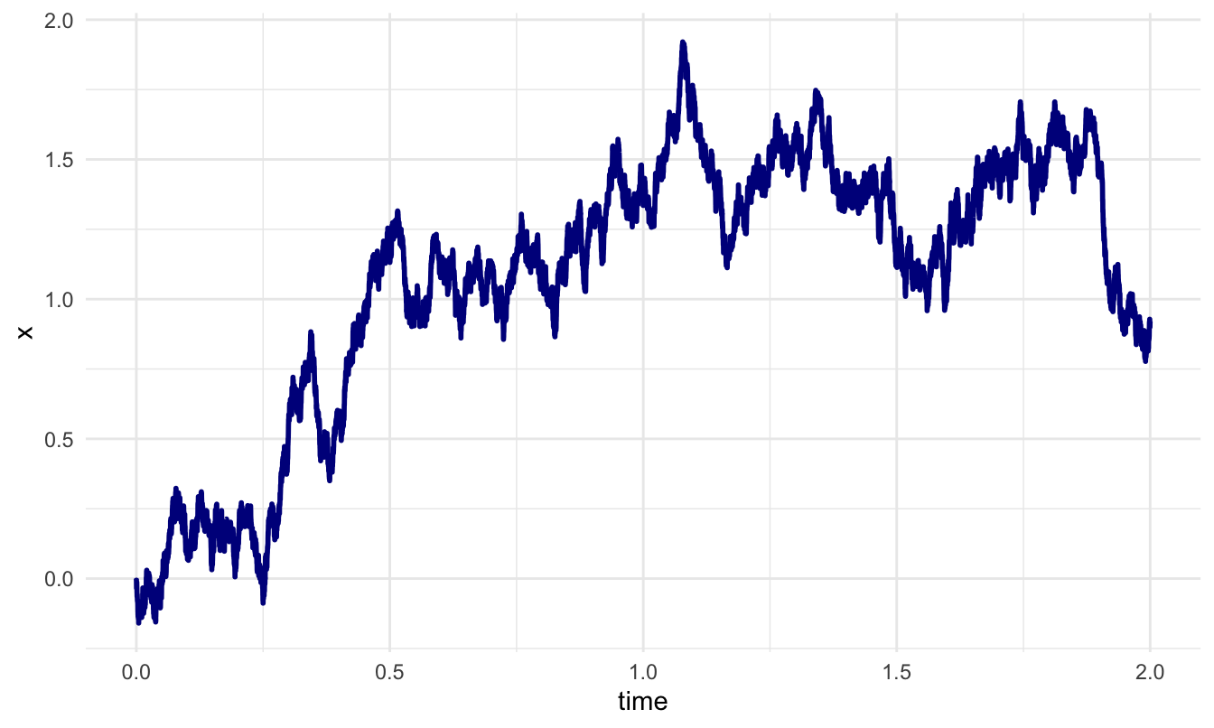
Wiener Diffusion Model

It is the expected distribution of the time until the process first hits or crosses one or the other boundary. This results in a bivariate distribution, over responses and hitting times.

• $\alpha$ : threshold
• $\beta$ : initial bias (starting point)
• $\delta$: quality of the stimulus (often $v$)
• $\tau$: non-decision time

Navarro & Fuss, 2009; Wabersich & Vandekerckhov, 2014. Copyright 2009, Joachim Vandekerckhove and Department of Psychology and Educational Sciences, University of Leuven, Belgium

Full Diffusion Decision Model

The Full DDM accounts for more behavioral phenomena by allowing trial-to-trial variability in key parameters:

Drift rate

Starting point

Non-decision time

Full DDM Parameters

$a$: decision boundary

$z$: starting point

$v$: drift rate

$t_0$: non-decision time

$s$: noise scale (usually fixed to 1)

$\eta$: SD of drift rate across trials

$s_{z}$: variability in start point

$s_{t_0}$: variability in non-decision time

Boehm, U., Annis, J., Frank, … & Wagenmakers, E. J. (2018). Estimating across-trial variability parameters of the Diffusion Decision Model: Expert advice and recommendations. Journal of Mathematical Psychology, 87, 46-75. Ratcliff, R., & Rouder, J. N. (1998). Modeling Response Times for Two-Choice Decisions. Psychological Science, 9(5), 347-356.

Purpose of variability

Adding variability improves the model’s ability to:

• Capture error RT differences
• Reflect trial-to-trial attention or difficulty changes
  

However, it increases computational demands.

Racing Diffusion Model

Instead of a single process choosing between boundaries, the RDM uses multiple independent diffusion processes, one per option. Each accumulator races toward its threshold. The first to cross wins. Tillman, Van Zandt, & Logan, 2020

Summary

Model	Core Mechanism	Key Strengths
Wiener	Noisy accumulation	Simple FPT, binary outcomes
Full DDM	Accumulation + param variability	Realistic RTs, error patterns
Racing DM	Multiple accumulators	Handles multi-alternative decisions

Core assumptions of the basic EAM

• Each decision = a single, continuous accumulation of evidence

• Culminates in a discrete response

• Evidence accumulates from stimulus onset to response

Guidelines

Boag et al. 2025

Within-Trial Stationarity

Model parameters are fixed within a trial

Evidence accumulation:

• Constant mean rate, though noisy
• No changes in stimulus evidence mid-trial

Decision thresholds:

• Set before stimulus onset
• Do not change during the trial

Within-Condition Stationarity

Parameters are constant across same-type trials

Assumes:

• Trials of same condition reflect same cognitive settings
• Participant behavior is stable

Free of contaminant processes

Data should reflect evidence accumulation!

Avoid:

• Random guessing

• Fast guesses

• Attention lapses or missing responses

Clean data = better model fit and interpretability.

“All models are wrong, but some are useful” - G. Box

Thank you!